Lecture 11: Generative Models and Reinforcement Learning

Week 6 · two surveys

Eoin O’Brien

Softmax with temperature

Decoding, revisited

• Last session: the decoder gives one logit per vocabulary item; softmax turns them into the next-token distribution
• After It takes great, over a toy vocabulary of 6 tokens:

	courage	care	skill	pride	the	banana
logit \(z_i\)	4.1	3	2.4	1.6	-0.5	-2
probability \(p_i\)	62%	21%	11%	5%	1%	<1%

• Observation: send a deployed language model the same prompt twice and the completions differ
  • a sampling setting named temperature controls by how much
• Held fixed: the trained weights and the prompt, hence the logits
• TRY: what could one number do to these logits to make the output more varied, or less?

• PROMPT: take guesses before the next slide. “Add noise” and “multiply them” both come up; multiplying is the right family.
• LISTEN FOR: “change the weights”. Nothing is retrained.
• The table is last session’s example, unchanged.

Softmax with temperature

Definition 1 The softmax with temperature divides every logit by a positive number \(\tau\), the temperature, before the softmax is applied.

\[ p_i = \frac{\exp\!\left(z_i/\tau\right)}{\sum_{j}\exp\!\left(z_j/\tau\right)}, \qquad \tau>0 \tag{1}\]

• Notation: \(z_i\) is the logit of token \(i\), \(p_i\) its probability, and the sum runs over the vocabulary (Hinton et al. 2015)
• Read aloud: divide every logit by \(\tau\), then take the softmax
• Shape: \(\tau\) is one scalar, shared by every logit
• At \(\tau=1\): the plain softmax of week 2 and last session
• Where it is set: in the sampler, at generation time; no weight changes
• Last session: attention divided every score by \(\sqrt{D_q}\) before its softmax, which is a fixed temperature of \(\sqrt{D_q}\)

• EMPHASIS: one number, outside the network. The logits are computed once and then divided.
• LISTEN FOR: “temperature is a hyperparameter of training”. For a language model it is a setting of the sampler.
• OPTIONAL: the name is from statistical physics, where the same formula gives the probability of a state from its energy.

The same logits at three temperatures

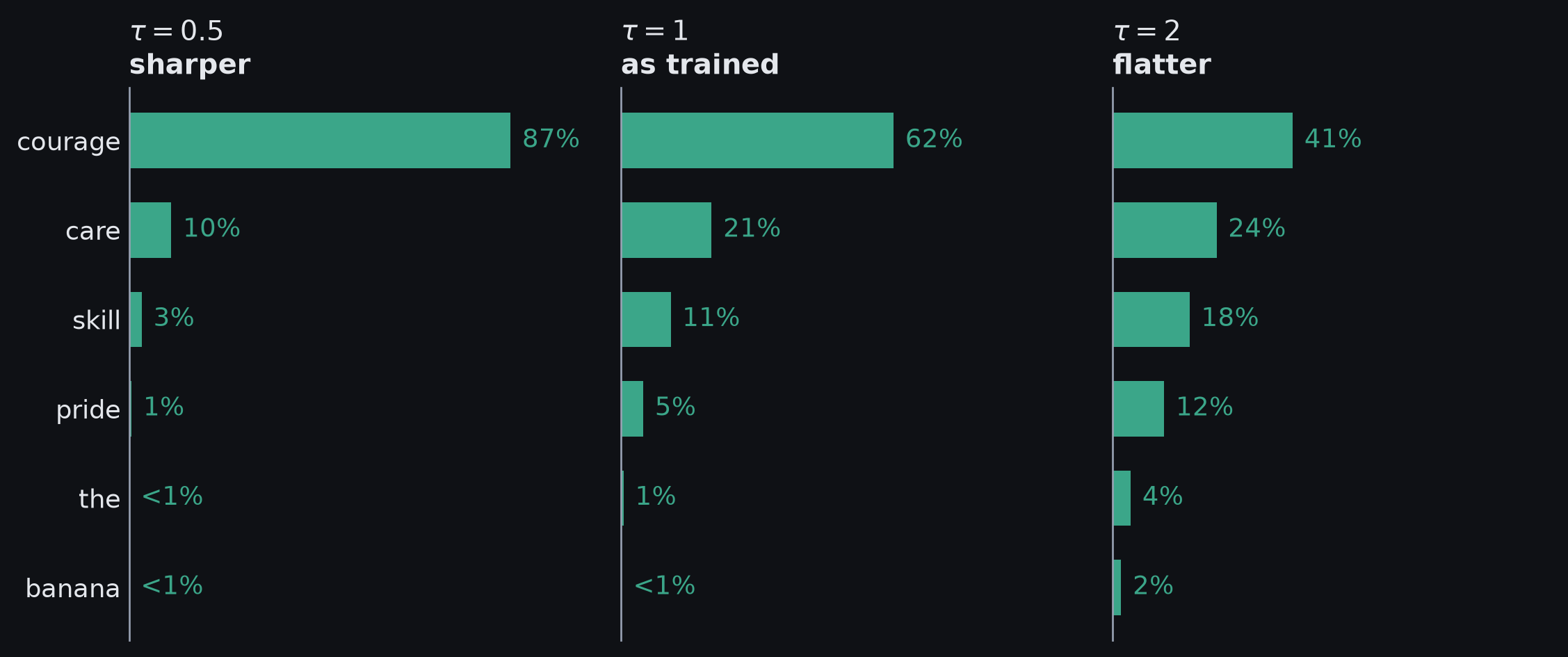
One set of logits, three temperatures. The tokens keep their order in every panel; what changes is how the probability is shared among them.

• PROMPT: before reading any numbers, which panel would you want for a tax return, and which for a poem?
• Point at banana: invisible on the left, a visible bar on the right.

The effect of temperature

	\(\tau=0.5\)	\(\tau=1\)	\(\tau=2\)
every gap between logits	multiplied by 2	unchanged	multiplied by 0.5
courage against care	9 times as likely	3 times	1.7 times
courage	87%	62%	41%
banana	one token in 230,000	one in 720	one in 51
a language model’s text	more predictable, generic	the distribution it was trained to output	varied, then incoherent

• As \(\tau\to0\): all the probability goes to the largest logit (greedy decoding)
• As \(\tau\to\infty\): every token gets the same probability, whatever its logit
• Temperature changes the samples without changing the model.

• EMPHASIS: the banana row. At the high setting a nonsense token arrives every few sentences, and each one becomes context for the next.
• LISTEN FOR: “high temperature makes the model more creative”. The model is unchanged; the sampler takes unlikely tokens more often.
• SOURCE: Prince’s notes to chapter 12 call greedy output generic and plain sampling degraded.

Temperature and ranking

• The ratio of any two probabilities depends only on the gap between their logits

\[ \frac{p_i}{p_j} = \exp\!\left(\frac{z_i-z_j}{\tau}\right) \tag{2}\]

• The ranking: a positive gap stays positive at every \(\tau\), so no token overtakes another
  • greedy decoding returns the same token at every temperature
  • temperature changes how often the sampler takes the second choice, never which token is second
• Against top-\(k\): two different operations on one distribution
  • temperature: every token reweighted, none removed
  • top-\(k\): the tail removed, the survivors kept in proportion
• Together: apply them in either order; temperature never changes the ranks top-\(k\) cuts on

• The ratio follows from Equation 1: the two sums cancel.
• PROMPT: at temperature two with top-three sampling, can banana appear? No: it is cut before or after, and the result is the same.

Quality and diversity

• A model that generates is two things
  • a learned distribution: the trained network
  • a sampling rule: how an output is drawn from that distribution
• Temperature belongs to the sampling rule; it trades one property of the samples for another
  • Lower: each sample more typical, the samples more alike
  • Higher: more variety, more poor samples
• Later today: the same trade appears when a GAN’s noise is truncated, when a diffusion model is guided, and when an agent explores

• This is the axis the generative survey is read on: how good is each sample, and how much of the data do the samples cover.
• DO NOT explain truncation, guidance or exploration here. Each gets its own slide.

Generative models

Unsupervised learning

• Until now: supervised learning, from pairs \(\{\vect{x}_i,\vect{y}_i\}\) and a loss that compares each output with its target
• Unsupervised learning: learning from the examples \(\{\vect{x}_i\}\) alone, with no labels
  • to generate new examples
  • to denoise, interpolate between or compress examples
  • to find structure, such as clusters, or to flag outliers

Definition 2 A generative model can synthesise new examples whose statistics are similar to those of its training data.

Definition 3 A probabilistic generative model is a generative model that also assigns a probability \(\prob{\vect{x}\mid\params}\) to any example \(\vect{x}\).

• Nested: every probabilistic generative model is a generative model; every generative model here is unsupervised
• The difference: a GAN generates but assigns no probability; flows, VAEs and diffusion models do both

• Today is the first goal on the list.
• LISTEN FOR: “generative means it uses probability”. A GAN is the counterexample. It is the next section.
• SOURCE: Prince section 14.1, figure 14.1.

Autoregressive models

• Last session’s decoder is a probabilistic generative model
  • No labels: the next token is its own target
  • Generates: sample a token, append it, repeat
  • Assigns a probability: to any sequence, by the chain rule

\[ \prob{t_1,\ldots,t_N} = \prob{t_1} \prod_{n=2}^{N} \prob{t_n\mid t_1,\ldots,t_{n-1}} \]

• Why it works: text has an order, so one hard distribution becomes a run of classifications over a vocabulary
• Cost: one pass through the network for every token generated
• An image: no natural order; a \(224\times224\) colour image is 150,528 numbers
  • ImageGPT generated pixel by pixel last session, which limited it to small images
• What else could turn something easy to sample into an image?

• This is the autoregressive family. It gets a row of its own in the comparison table at the end of the survey.
• SOURCE: Prince section 14.1, the footnote on the transformer decoder.
• PROMPT: let the closing question hang. The next slide answers it.

Latent variables

• Idea: draw some random numbers and let a network turn them into an example
  1. draw \(\vect{z}\) from a simple distribution \(\prob{\vect{z}}\), usually a standard normal
  2. map \(\vect{z}\) to the data space with a network

Definition 4 A latent variable \(\vect{z}\) is a variable the model uses to explain an example \(\vect{x}\) but that is never observed in the data.

• Size: in GANs and VAEs \(\vect{z}\) has fewer entries than \(\vect{x}\), a compressed description of it
  • in flows and diffusion models it is the same size as \(\vect{x}\)
• Not a label: a label was recorded for each training example; no \(\vect{z}\) was recorded for any
• Notation: last session \(\vect{z}\) was a vector of logits; from here on it is a latent variable
• All four families today generate this way

• EMPHASIS: step one is easy on purpose. All the learning is in step two.
• LISTEN FOR: “z is the class of the image”. Nothing was observed; the model invents z.
• SOURCE: Prince section 14.1. Same-size latents: section 16.2 for flows, the opening of chapter 18 for diffusion.

The pairing problem

• Supervised: every input \(\vect{x}_i\) arrived with its target \(\vect{y}_i\); the loss compared the network’s output with it
• Now: the network takes \(\vect{z}\) and outputs an example; the training set holds only examples \(\vect{x}_i\)
  • draw one \(\vect{z}\): which training example should it become?
  • nothing says, so this \(\vect{z}\) has no target and no per-example loss
• With no pairing between noise and data, what is the training signal?
• Each of the four families that follow answers that question, at a cost
• TRY: propose one

• PROMPT: give this a full minute in pairs. Expect “compare to the nearest training image” and “train a classifier to tell them apart”. The second is the next section.
• Nearest-training-image is worth a sentence: it rewards memorising the training set.
• EMPHASIS: this question is the thread for the next four sections. Return to it by name at the start of each family.

Fitting a generative model

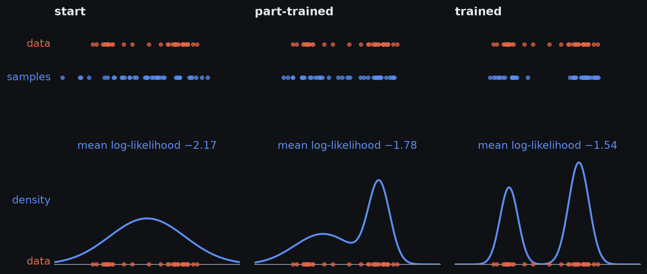
One model at three stages of training, seen two ways. Top: the samples it generates, beside the data. Bottom: the density it assigns, over the same data.

• After Prince figure 14.2, redrawn on one model so the two rows can be compared.
• The model is a mixture of two Gaussians. How it is being moved is not the point; DO NOT explain the fitting algorithm.
• PROMPT: in the top row, how would you measure that the right-hand panel is better than the left without the bottom row?

Fitting: samples and likelihood

• From the samples, the figure’s top row: make generated samples indistinguishable from real examples
  • no probability is needed, only a way to tell the two sets apart
  • GANs
• From the density, the bottom row: make the training examples probable under the model
  • flows, VAEs and diffusion models

\[ \loss[\params] = -\sum_{i=1}^{I}\log\prob{\vect{x}_i\mid\params} \tag{3}\]

• Read: week 2’s negative log-likelihood, with examples and no targets
• One budget: a distribution sums to one, so raising the probability of the data lowers it everywhere else
• Beyond training: a probability compares two models on held-out data and flags an outlier

• The printed number in each bottom panel is this loss, sign flipped and averaged over the examples.
• LISTEN FOR: “why not just make the density huge at each training point?” That is overfitting; it is why the comparison is made on held-out data.
• SOURCE: Prince section 14.1, equation 14.1.

Desirable properties

• Efficient sampling: a new sample is cheap to generate; many can be made in parallel
• Sample quality: samples can’t be told from the real data
• Coverage: samples represent the whole training distribution, not a subset of it
• Well-behaved latent space: every \(\vect{z}\) gives a plausible example; a small change in \(\vect{z}\) gives a small change in the example
• Disentangled latent space: each entry of \(\vect{z}\) controls one interpretable property
• Efficient likelihood: the probability of a new example is cheap to compute and accurate
• No family has all six.
• Temperature traded quality against coverage within one model; the families trade them against each other

• These six are the columns of the comparison table at the end of the survey. Students should be able to name them.
• PROMPT: which two did temperature trade against each other? Quality and coverage.
• The individual assignments are disputable. Say so.
• SOURCE: Prince section 14.2, figure 14.3.

Generative adversarial networks

Discrimination as a signal

• Which \(\vect{z}\) should become which \(\vect{x}\)? A GAN doesn’t pair them at all
• No generated sample can be scored against a target, because it has none
• A classifier can still be trained to tell generated samples from real examples
  • If it succeeds: whatever tells them apart is a signal for changing the samples
  • If it fails: the samples can’t be told from the data, the original goal
• The classifier is trained on the two sets; no sample is matched to any example
• Name: generative adversarial network, or GAN (Goodfellow et al. 2014)

• Return to the pairing problem by name. This is the proposal some of the room will have made a few slides ago.
• EMPHASIS: the classifier is a means. Nobody wants it at the end.
• SOURCE: Prince section 15.1.

Generator and discriminator

Definition 5 The generator is a network that maps a latent variable \(\vect{z}\), drawn from a simple distribution, to a sample \(\vect{x}^{*}\).

Definition 6 The discriminator is a network that takes an example and outputs an estimate of the probability that it is real rather than generated.

• The discriminator’s task: week 2’s binary classification, with real as 1 and generated as 0
• The generator’s task: change its parameters so the discriminator is less confident that its samples are generated
• One loss, two players: the discriminator lowers it, the generator raises it, and the updates alternate
• If training succeeds: the discriminator outputs one half for everything
  • it is then thrown away
• What the generator sees: never a real example, only the discriminator’s gradient

• The ring run two slides on uses the generator’s usual non-saturating loss, which is not literally the same loss with the sign flipped.
• No equation here by design. The loss is binary cross-entropy; Prince’s equation 15.2 to equation 15.5 write it out for anyone who wants it.
• LISTEN FOR: “the generator copies training images”. It has never been shown one.
• OPTIONAL: the technical name for the end state is a Nash equilibrium, a point that is a minimum for one player and a maximum for the other.

A one-dimensional GAN

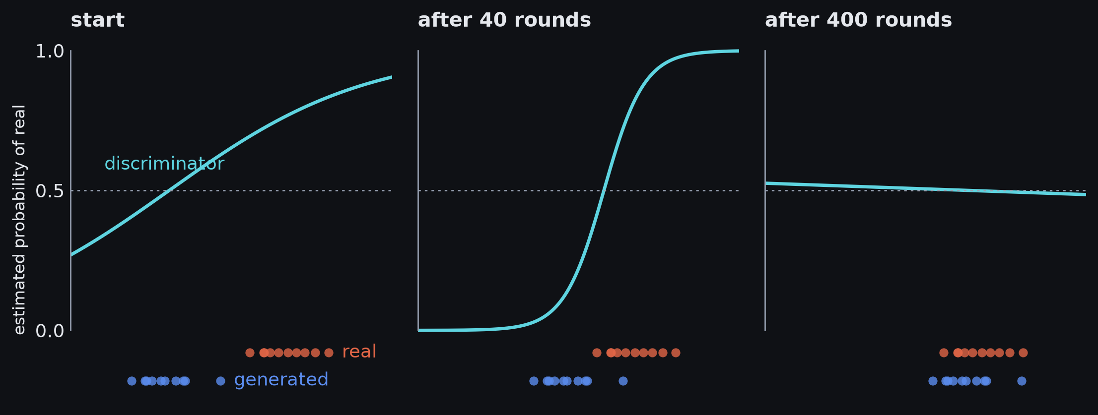
A GAN small enough to watch. The generator adds one learned number to its noise, which slides its samples along the axis; the discriminator is a sigmoid of position.

• The notebook for this section plays the same game.
• SOURCE: Prince section 15.1, equation 15.1, figure 15.1.
• PROMPT: before advancing, which way will the generated samples move, and what tells them to?

A one-dimensional GAN: training

• Start: the generated samples sit left of the real examples; the discriminator has begun to rate the right as real
• The push: the generator moves its samples the way the curve rises
• After 40 rounds: the samples have moved; the discriminator still separates them, more sharply
• After 400 rounds: the two sets overlap; the curve is flat at one half
  • a flat curve has no slope, so the push has gone
  • on the way the samples overshot the data, then came back
• The end state is a balance between two networks, not a loss driven to zero.
• Consequence: neither network’s loss, falling, says that training is going well

• The overshoot is in the run, not in the three panels: the generator’s shift passes the real mean and returns.
• LISTEN FOR: “so we train until the loss is small”. Whose loss? Each player’s gain is the other’s loss.

Mode collapse

• Mode: a peak of the data distribution, one kind of example
• What the discriminator scores: one sample at a time; it never sees the spread of a batch
• A generator can fool it with one accepted sample, returned for every \(\vect{z}\)

Definition 7 Mode collapse is the failure in which a generator ignores most of the variation in its latent variable and produces only one or a few distinct samples.

• Mode dropping: the milder case, plausible samples that cover only part of the data
  • a face generator that never produces a beard
• Property lost: coverage
• Why it goes unnoticed: with no probabilities, nothing reports that part of the data is never generated

• SOURCE: Prince section 15.1.4.
• PROMPT: how would you detect mode dropping in a face generator with ten thousand samples and no labels? Hold the answers for the evaluation section.

Mode collapse on a ring

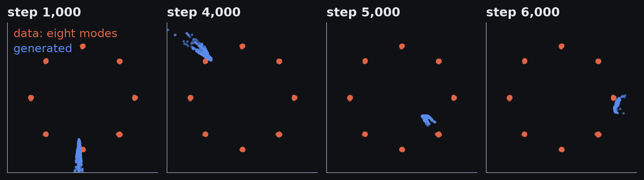
One small GAN at four chosen points in training, on data with eight modes. The generated clump is narrow and moves; it never settles on the data. The run was set up to fail: its discriminator learns ten times more slowly than its generator.

• In each panel every sample has the same nearest mode, a different one each time. The clump is near that mode, not on it: this run fails on quality as well as coverage.
• The four steps are chosen. At the recorded steps between them the clump is split across two neighbouring modes.
• PROMPT: why does the clump move? The discriminator learns to call that region generated, so the generator leaves for a mode the discriminator hasn’t caught up with.
• LISTEN FOR: “GANs always do this”. This run was set up to fail. With the generator slowed to the discriminator’s learning rate, the same networks spread their samples round the whole ring, though many fall between the modes.

Vanishing gradients

• TRY: in the one-dimensional game, suppose the discriminator is trained to perfection before the generator moves at all. What is its curve where the generated samples sit?
• Flat, at zero: a small change to the generator changes none of the discriminator’s outputs
• The generator’s gradient vanishes when its samples are at their worst
  • against a perfect discriminator, samples 6 standard deviations from the data get 3% of the push that samples 2 away get
• Last session: a saturated softmax gave near-zero gradients; a saturated sigmoid does the same here
• The balance: too weak a discriminator gives no useful signal; too strong a one gives no gradient
• In practice: a GAN is sensitive to choices of architecture, activation and optimiser that most networks tolerate

• The computed line uses unit-variance real and generated distributions and the best possible discriminator for them.
• The DCGAN’s choices: strided convolutions, BatchNorm placement, leaky ReLU in the discriminator, lowered Adam momentum.
• DO NOT introduce the Wasserstein distance. It is the standard repair, but it is not taught.
• SOURCE: Prince section 15.2.2; section 15.1.4 for the DCGAN.

Truncation

• A sampling-time rule: draw \(\vect{z}\) and reject it if it lies further than a threshold from the mean of its distribution
• Tight threshold: higher average quality, less variety
• Loose threshold: more variety, more defects
• Very tight: samples that look almost identical
• Truncation does to \(\vect{z}\) what a low temperature does to logits
  • the trained generator is unchanged
  • quality is bought with diversity

• Truncation is the second control that trades quality against diversity. Say so.
• Prince writes the threshold as tau, which this deck keeps for temperature.
• SOURCE: Prince section 15.3, figure 15.10, after Brock et al. (2018).

GANs: trade-offs

Buys	Gives up
high-quality samples	any probability for an example
one pass through the generator per sample	stable training
a well-behaved latent space	coverage

• Pairing: none; a second network judges the samples against the data

• This two-column shape repeats for each family. The cells are drawn from the six desirable properties.
• SOURCE: Prince figure 14.3, the GAN row.

Normalising flows

Invertible maps

• Which \(\vect{z}\) should become which \(\vect{x}\)? A flow makes the map one-to-one, so every \(\vect{x}\) has exactly one \(\vect{z}\)
• Generating: draw \(\vect{z}\) and compute \(\vect{x}=\mathrm{f}[\vect{z},\params]\), as in a GAN
• The new constraint: the network can be run backwards, \(\vect{z}=\mathrm{f}^{-1}[\vect{x},\params]\)

Definition 8 A normalising flow is a probabilistic generative model that transforms a simple base density over a latent variable \(\vect{z}\) into a density over the data, using a network that is invertible.

• Consequence: each training example traces back to its one latent; the pairing is computed, not guessed
• Name: run backwards, the network turns the data’s distribution into a normal one (Rezende and Mohamed 2015)

• Return to the pairing problem by name. The GAN avoided it; the flow removes it by construction.
• LISTEN FOR: “any network can be inverted if you train a second one to undo it”. That is the next family. Here the inverse is exact, by design of the layers.
• SOURCE: Prince section 16.1, 16.1.2.

Transforming a density

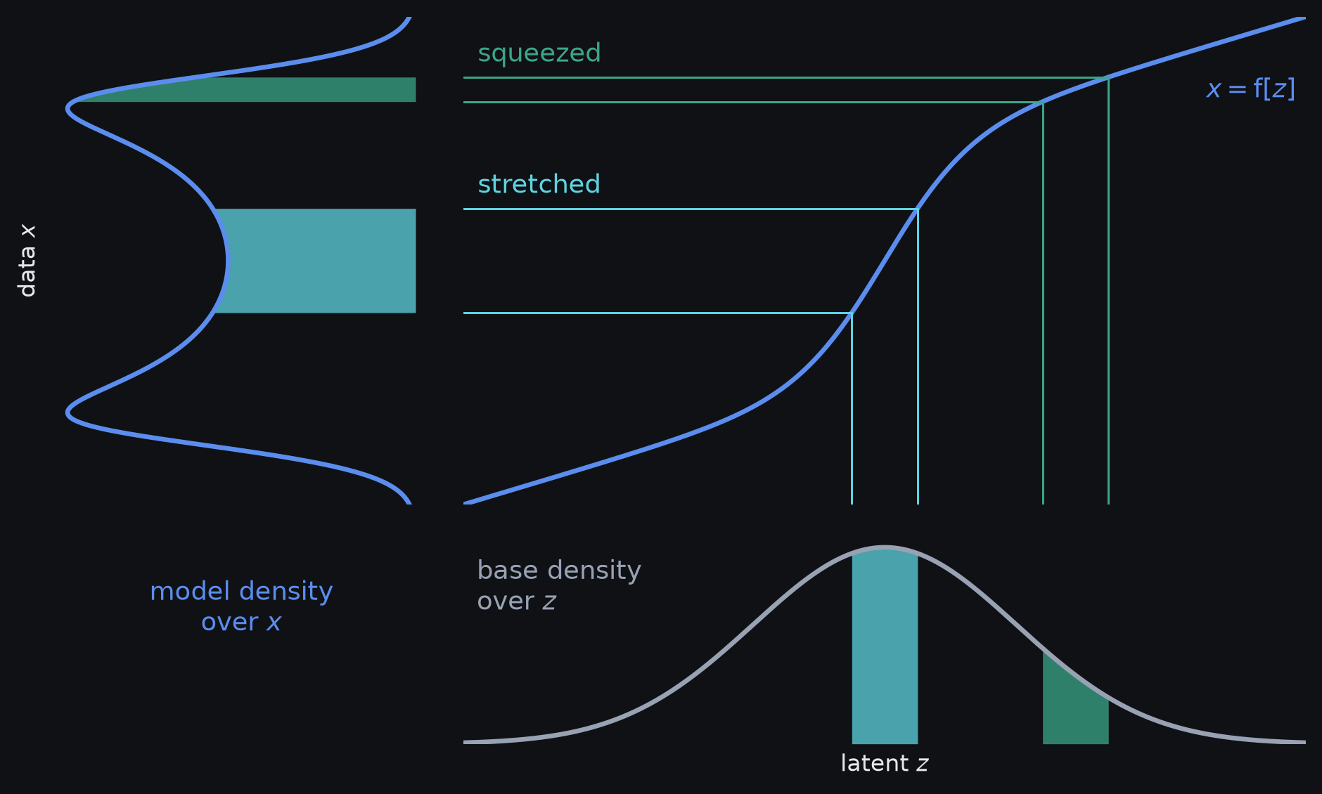
A flow in one dimension. A standard normal over the latent, bottom, passes through an invertible map, top right, and becomes the model’s density over the data, left. Each shaded strip holds the same probability before the map and after it.

• The map is chosen by hand to make two modes; nothing here is trained. In a real flow the map is a network and its parameters are learned.
• PROMPT: the stretched strip is wider on the left than at the bottom. What must have happened to its height?
• After Prince figure 16.1 and figure 16.2.

The density under a map

• Conserved: the probability in a strip of \(z\) equals the probability in the strip of \(x\) it maps to
• Stretched strip: the map is steep; the same probability covers 2.7 times the width, so the density is lower
• Squeezed strip: the map is shallow; the width shrinks to 0.62 of what it was, so the density is higher

\[ \prob{x\mid\params} = \left|\frac{\partial\,\mathrm{f}[z,\params]}{\partial z}\right|^{-1} \prob{z}, \qquad z=\mathrm{f}^{-1}[x,\params] \tag{4}\]

• Read aloud: the density at \(x\) is the base density at its latent, divided by how much the map stretches there
• In more dimensions: the stretch of a length becomes a change of volume; the statement is otherwise the same
• The probability of any example is exact.
  • training is the negative log-likelihood of Equation 3, with nothing approximated

• This is the one equation of the section. Read it once in words and move on; DO NOT derive it.
• The inverse is needed to find z for a given x, which is why the layers must be invertible, not just the map in principle.
• OPTIONAL: the volume change is the determinant of the Jacobian. Named for anyone who meets it in the reading.
• SOURCE: Prince section 16.1.1, equation 16.1.

Flows: trade-offs

Buys	Gives up
the exact probability of any example	architectural freedom: every layer must be invertible, with a stretch that is cheap to compute
the latent of any example, by running backwards	compression: \(\vect{z}\) is as large as \(\vect{x}\)
ordinary maximum-likelihood training	sample quality, behind GANs and diffusion models

• Pairing: by construction; an invertible map pairs every example with one latent

• Much of the research on flows is the search for layers that are invertible, expressive and cheap.
• SOURCE: Prince section 16.2.2 for the requirements on layers; figure 14.3, the flows row.

Variational autoencoders

A latent variable model

• Which \(\vect{z}\) should become which \(\vect{x}\)? A variational autoencoder leaves the network unconstrained and trains a second network to guess
• First, a way to describe \(\prob{\vect{x}}\) in two simple pieces
  • how the latent is distributed, the prior \(\prob{\vect{z}}\)
  • how an example depends on the latent, \(\prob{\vect{x}\mid\vect{z}}\)

Definition 9 A latent variable model describes \(\prob{\vect{x}}\) indirectly: it models the joint distribution \(\prob{\vect{x},\vect{z}}\) of the data and a latent variable, and obtains \(\prob{\vect{x}}\) by marginalising over \(\vect{z}\).

• Marginalising: adding up \(\prob{\vect{x}\mid\vect{z}}\prob{\vect{z}}\) over every value \(\vect{z}\) could take
• A mixture of Gaussians: \(z\) picks one of a few components, each a simple bump
• The step up: \(\vect{z}\) is continuous; a network turns it into the mean of a Gaussian over \(\vect{x}\)
  • a mixture with infinitely many components

• Return to the pairing problem by name: the flow made the pairing computable by restricting the network. This family refuses the restriction.
• EMPHASIS: simple pieces, complicated total. The next slide is the picture.
• SOURCE: Prince section 17.1 and section 17.2.

Mixtures of Gaussians

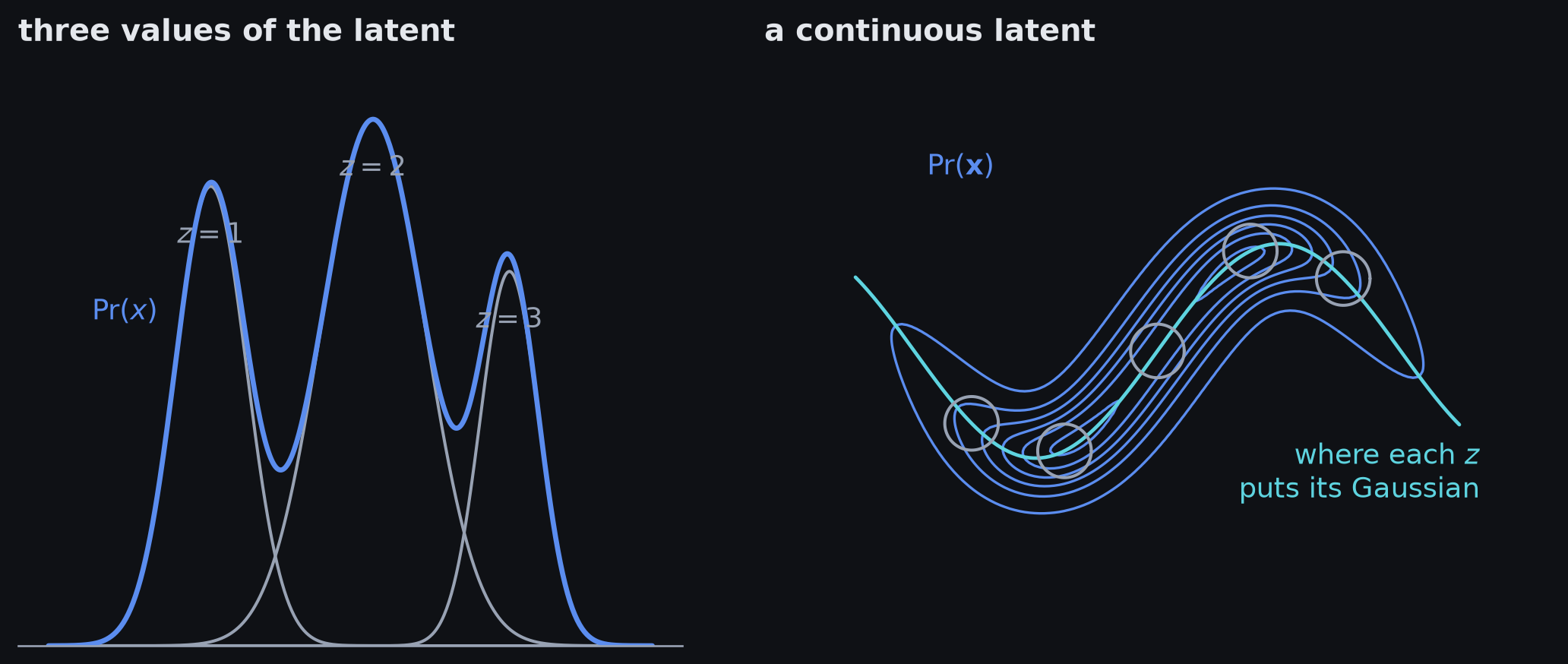
Left: a latent with three values, each choosing one Gaussian; the density is their weighted sum. Right: a continuous latent, each value placing a small round Gaussian along a curve; the contours are the density they add up to.

• Right-hand panel: the curve is drawn by hand here. In a variational autoencoder the decoder computes it.
• PROMPT: no single Gaussian on the right is curved. Where does the curved shape come from?
• After Prince figure 17.1 and figure 17.2.

The intractable likelihood

• Maximum likelihood needs \(\prob{\vect{x}_i}\) for every training example
• With a continuous latent that is a sum over every possible \(\vect{z}\), each one passed through a deep network
  • no closed form
  • no easy way to evaluate it for one particular \(\vect{x}\)
• Most latents are irrelevant: for a given \(\vect{x}\), almost every \(\vect{z}\) decodes to something unlike it, so it adds almost nothing to the sum
• The idea: train a second network to propose, for each \(\vect{x}\), the few \(\vect{z}\) that matter
• The price: training maximises a lower bound on the log-likelihood, not the log-likelihood itself

• The pairing problem again, in probabilistic terms: “which z made this x?” has no computable answer, so it is approximated.
• Prince writes the sum as an integral, equation 17.9.
• SOURCE: Prince section 17.3.

Encoder and decoder

Definition 10 A variational autoencoder pairs two networks and trains them together: a decoder that maps a latent variable \(\vect{z}\) to the mean of \(\prob{\vect{x}\mid\vect{z}}\), and an encoder that maps an example \(\vect{x}\) to the mean and variance of \(q(\vect{z}\mid\vect{x})\), a normal distribution that approximates the posterior \(\prob{\vect{z}\mid\vect{x}}\).

• Decoder: latent in, mean of a Gaussian over examples out; with the prior, this is the model
• Encoder: example in, a normal distribution over latents out; the learned guess at the pairing
• Posterior: the distribution of the latents that could have produced this example
• Autoencoder: a network trained to reproduce its input through a narrow middle layer
  • its encoder outputs one point: compression, but no distribution to sample from
• After training: new examples need the prior and the decoder only

• \(q\) is a new letter on purpose: it is an approximation, not a distribution the model defines.
• LISTEN FOR: “the encoder is the generative model”. The encoder is scaffolding for training; generation never calls it.
• SOURCE: Prince section 17.6; the introduction (Kingma and Welling 2013).

Encoder and decoder: one training step

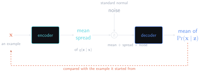
One training step of a variational autoencoder. The encoder proposes a distribution over latents for this example; one latent is drawn from it using noise from a side branch; the decoder turns that latent back into an example.

• Walk it left to right once, then point at the dashed line: the example is its own target.
• The side branch is the subject of the slide after next. Park questions about it.
• After Prince figure 17.9 and figure 17.11.

The evidence lower bound

Definition 11 The evidence lower bound (ELBO) is a function of the encoder’s and decoder’s parameters that is less than or equal to the log-likelihood \(\log\prob{\vect{x}}\) of an example, for every setting of those parameters.

\[ \operatorname{ELBO} = \expectsub{q(\vect{z}\mid\vect{x})}{\log\prob{\vect{x}\mid\vect{z}}} - \kl{q(\vect{z}\mid\vect{x})}{\prob{\vect{z}}} \tag{5}\]

• Read aloud: how well the decoder rebuilds \(\vect{x}\) from the encoder’s latents, minus how far the encoder’s distribution is from the prior
• Evidence: another name for the likelihood of the data
• Lower bound: training raises it; the log-likelihood can never be below it
  • the gap between the two is not measured
• Notation: the two networks’ parameters are left out of the symbols here; Prince writes them
• Stated, not derived: Prince section 17.3 has the derivation

• This is the one equation of the section. Read it in words; DO NOT derive it and DO NOT introduce Jensen’s inequality.
• SOURCE: Prince equation 17.21, with his integral written as an expectation.

The evidence lower bound: two terms

• Reconstruction, the first term: with a Gaussian decoder it is a negative squared error between the example and the decoder’s output, scaled, plus a constant
• Regularisation, the second term: week 2’s KL divergence, pulling every example’s latents towards the one prior
  • so a latent drawn from the prior decodes to something sensible
• The tension
  • perfect reconstruction: each example’s latents sit in a private corner far from the prior
  • a perfect match to the prior: the latents say nothing about the example
• On the digits model: per image, reconstruction 20, minus a KL of 5, gives a bound of 15
  • for continuous data the model assigns a density, whose log can be positive

• PROMPT: which term would you drop to get a plain autoencoder? The second. What do you lose? The ability to sample.
• The numbers are in nats and mean little on their own; the point is that the bound is two measurable quantities.

Reparameterisation

• The problem: a training step draws a random \(\vect{z}\) in the middle of the network; backpropagation can’t pass through a random draw to reach the encoder
• The idea: draw standard-normal noise on a side branch, then compute the latent from it
  • latent = mean + spread × noise
• Same distribution: the result is still a draw from the encoder’s normal
• What changed: the randomness is an input; the path from the encoder to the loss is ordinary arithmetic
• Later today: diffusion models write a noisy example the same way

• Point back at the diagram: the noise arrow enters from above, and no gradient needs to travel up it.
• SOURCE: Prince section 17.7, equation 17.25.

The latent space

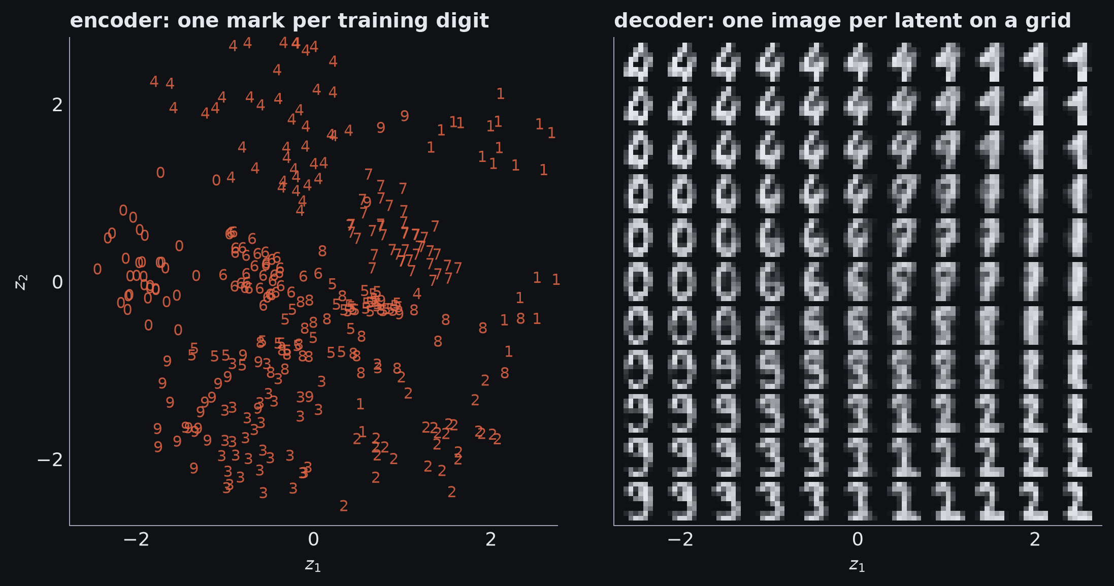
A variational autoencoder with a two-dimensional latent, trained on small handwritten digits. Left: where the encoder places training digits, each marked by its label, which the model never saw. Right: what the decoder draws at each point of a grid over the same space.

• Neighbouring latents decode to similar images, and the digit classes have settled into regions without any label being shown.
• PROMPT: pick a point halfway between the fours and the ones. What does the decoder draw there?
• Two latent dimensions is far too few for good digits. It is chosen so the whole space fits on a slide.
• The digits are the 8 by 8 optical-recognition set that ships with scikit-learn.

Reconstructions

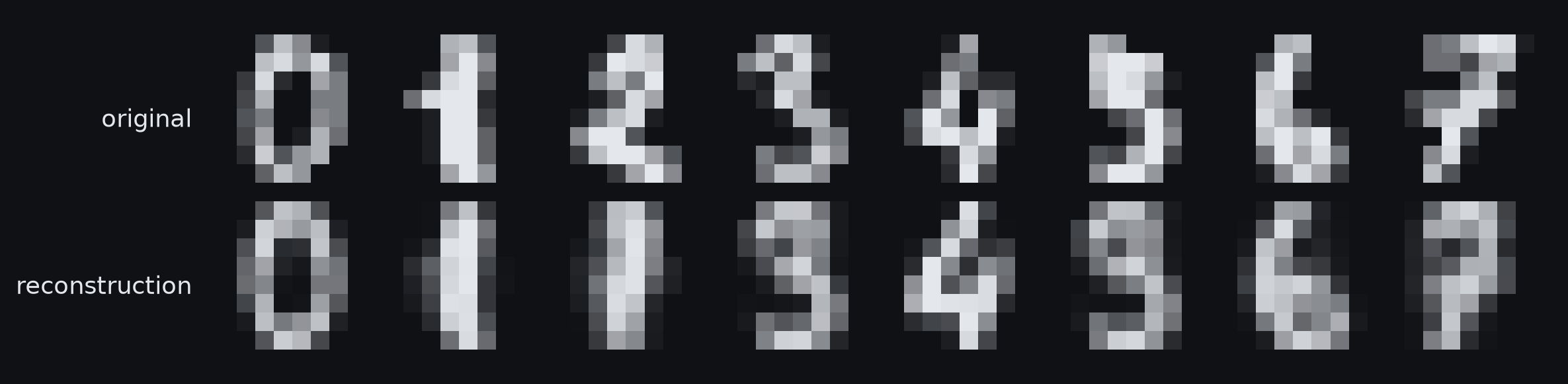
Eight training digits, and below each the image the decoder returns from the encoder’s mean latent for it.

• The reconstructions are blurred, and some have drifted towards a neighbouring digit.
• Part of this is the two-dimensional latent. Part is general: blur comes partly from the Gaussian decoder and partly from the approximate encoder.
• SOURCE: Prince, notes to chapter 17.

VAEs: trade-offs

Buys	Gives up
any decoder architecture	the likelihood itself: only a lower bound on it is known
a compressed latent space in which nearby points decode alike	sharpness: samples and reconstructions are typically blurry
an encoder, as a by-product

• Pairing: learned; a second network learns, for each example, which latents could have made it

• SOURCE: Prince figure 14.3, the VAE row.

Diffusion models

The diffusion process

• Which \(\vect{z}\) should become which \(\vect{x}\)? A variational autoencoder learned an encoder to guess; a diffusion model fixes the encoder in advance, so it needs no training
• Forward process: blend the example with a little Gaussian noise and repeat until only noise is left
  • nothing is learned here

Definition 12 A diffusion model has a fixed forward process, which turns an example \(\vect{x}\) into noise through a series of latent variables \(\vect{z}_1,\ldots,\vect{z}_T\) by blending in a little Gaussian noise at each step, and a learned reverse process, which removes that noise one step at a time.

• Latents: every noisy version \(\vect{z}_t\), each the same size as \(\vect{x}\)
• Free pairs: for any training example we can make a noisy version and know exactly what noise went in
  • an input and a target, for one step
• Reverse process: a network that undoes one step (Sohl-Dickstein et al. 2015; Ho et al. 2020)

• Return to the pairing problem by name: the GAN avoided it, the flow computed it, the VAE learned it. This family manufactures it.
• The pair has changed: it is a noisy version and its noise, not a latent and an example. Which pure noise ends as which example is still unassigned; the reverse path settles it.
• EMPHASIS: the forward process has no parameters. All the learning is in the reverse direction.
• The forward process is the encoder and the reverse process the decoder. That is the link back to the last section.
• SOURCE: Prince section 18.1, figure 18.1.

Forward and reverse processes

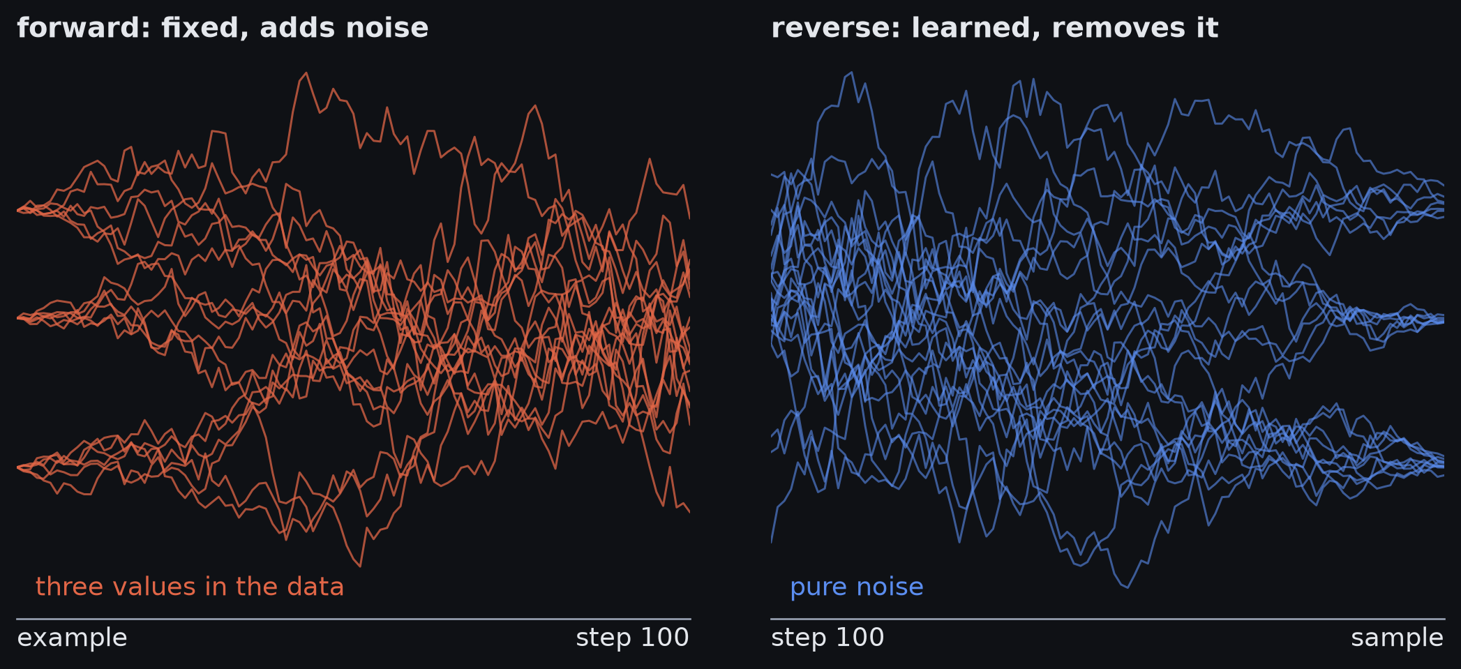
Diffusion on one-dimensional data that takes three values. Left: the fixed forward process carries examples into noise. Right: a trained network run backwards from pure noise, whose paths end on the three values.

• Left: no network. Right: the same network applied at every step.
• All three values are reached, in close to the data’s proportions. Worth saying, after mode collapse.
• PROMPT: on the right, when does a path “decide” which value it will end on? Not at the start.
• After Prince figure 18.1 and figure 18.2.

Small steps

• All at once: turning pure noise into an example in one step is the original problem
• One small step: given \(\vect{z}_t\), the version one step earlier is nearly Gaussian, centred on a point a network can predict
• Generating: start from pure noise; \(T\) times, take the predicted step and add a little fresh noise
  • \(T=100\) in the figure’s model
• One network: shared by every step, with the step number as an extra input

• This is the idea that makes the reverse direction learnable. Slow down here.
• LISTEN FOR: “the network removes all the noise each time”. It removes one step’s worth.
• SOURCE: Prince section 18.7.

Noise prediction

• A training step: take an example, pick a step \(t\), add that much noise, and ask the network what noise was added

\[ \loss = \sum_{t=1}^{T} \norm{\vect{g}_t[\vect{z}_t]-\noise_t}^{2} \tag{6}\]

• Notation: \(\vect{z}_t\) is the noisy version at step \(t\), \(\noise_t\) the noise that was added, and \(\vect{g}_t\) the network at that step
• Read aloud: the squared distance between the noise the network predicts and the noise that was added
• Week 1: the least-squares loss, with noise as the target

• The one equation of the section, stated and read. DO NOT derive it and DO NOT introduce the noise schedule’s symbols.
• SOURCE: Prince section 18.5, equation 18.40, without its sum over examples.

Noise prediction: origin of the loss

• Reparameterisation: the noisy version is the example scaled down plus noise scaled up, so the noise is a known input

• Where it comes from: an evidence lower bound, as for the variational autoencoder; with the encoder fixed and per-step weights dropped, it simplifies to this

• Scope: written for one example; training also sums over the examples

• Training a diffusion model is ordinary regression.

• EMPHASIS: after an adversarial game and a bound with two competing terms, this is plain regression. That is the family’s practical appeal.
• SOURCE: Prince section 18.7.

Diffusion: trade-offs

Buys	Gives up
high-quality samples	sampling speed: many network passes per sample; the other three take one
stable training, with a plain least-squares loss	a compact latent: each \(\vect{z}_t\) is as large as \(\vect{x}\), with no organisation by meaning

• Mitigation: samplers that skip steps
• Pairing: manufactured; known noise is added to real examples

• Coverage is a question mark for this family in the comparison table, as for flows and VAEs. Don’t claim it.
• SOURCE: Prince figure 14.3, the diffusion row; section 18.6.2 for faster samplers.

Conditional generation

Conditioning

• A sample from \(\prob{\vect{x}}\) is some example, but a user wants a particular kind

Definition 13 Conditional generation draws samples from \(\prob{\vect{x}\mid\vect{c}}\), where \(\vect{c}\) is information supplied with the request, such as a class label or a text prompt.

• Mechanism, in every family: give the condition to the network as an extra input and train on examples that each come with their condition
• Conditional GAN: the generator and the discriminator both receive the label
• Text to image: the condition is a language model’s embedding of the prompt
• Last session: a language model’s prompt is a condition too; the next-token distribution is conditioned on the text so far

• The condition is not a latent: it is observed and supplied by the user.
• SOURCE: Prince section 15.4.1 for the conditional GAN; section 18.6.3 and figure 18.11 for text-conditioned diffusion.

Guidance

• Training: one diffusion model, given the condition on most examples and denied it on the rest
  • so it can denoise with the condition or without it
• Sampling: take each step further in the direction the condition adds than the model alone would
  • a strength of zero is the plain conditional model
• More guidance: samples match the condition more closely and vary less
  • the results are very high quality but slightly stereotypical (Prince 2023)
• Guidance trades diversity for quality, as temperature does for text and truncation for a GAN
• Name: classifier-free guidance (Ho and Salimans 2022)

• The earlier variant, classifier guidance, uses the gradient of a separate classifier to push each step towards the class. Named only.
• SOURCE: Prince section 18.6.3, including the analogy to truncation.
• OPTIONAL: high-resolution systems chain several diffusion models, a small image first and then models that enlarge it.

Guidance at three strengths

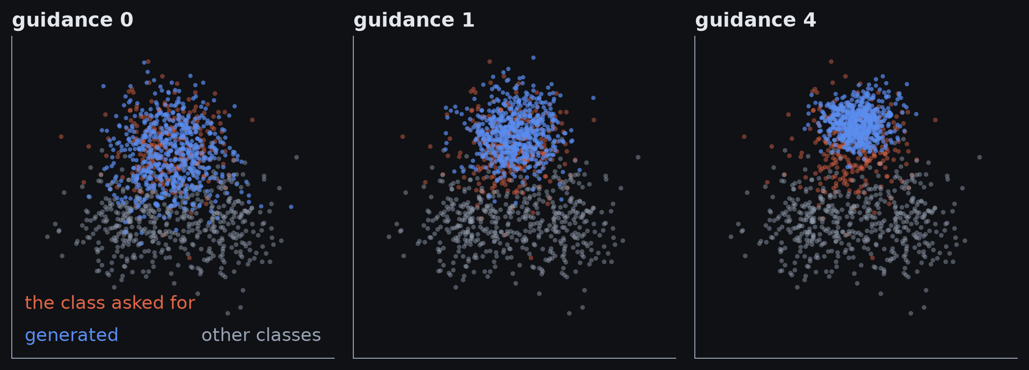
A diffusion model on three overlapping classes, asked for one of them at three guidance strengths. With more guidance the samples leave the region shared with the other classes, and bunch together.

• At the highest strength the samples sit beyond the class’s own centre, away from the other two: more typical of the class than the class is.
• PROMPT: which panel has the best precision? Which has the best recall? Hold the terms until the evaluation section.
• After figure 2 of Ho and Salimans.

Evaluating generative models

Test likelihood

• No labels, so no accuracy: how is one generative model shown to be better than another?
• For a probabilistic model: the likelihood it gives to held-out examples
• Why not the training set: a model that memorises puts all its probability on the training examples, so it can generate nothing else
• What the test set rewards: generalisation and coverage together
  • a model that covers part of the data must give the rest low probability
• Who can report it
  • flows and last session’s decoder: exactly
  • VAEs and diffusion models: a lower bound only
  • GANs: not at all
• Week 3: training error against test error, with likelihood in place of error

• LISTEN FOR: “just look at the samples”. That checks quality on the handful you looked at. It says nothing about coverage.
• OPTIONAL: test likelihood is what a language model’s perplexity reports; no equivalent exists for a GAN.
• SOURCE: Prince section 14.3.

Fréchet inception distance

Definition 14 The Fréchet inception distance (FID) is a distance between the distribution of generated samples and the distribution of real examples, computed on the features of a pretrained image classifier, with each distribution approximated by a multivariate normal.

• Idea: compare real and generated images by what a trained classifier makes of them, not pixel by pixel
• Reading it: lower is better; zero means the two normal summaries are identical
• Needs no probability, so it applies to every family, GANs included (Heusel et al. 2017)
• Limits
  • images only
  • anything the classifier’s features discard can’t affect the score
  • one number mixes realism and diversity
• Inception score: an earlier measure built on the same classifier, with the same dependence

• “Inception” is the name of the classifier whose features are used.
• A model that is sharp but narrow and one that is broad but flawed can score the same. The next slides separate the two.
• DO NOT write out the inception score’s formula.
• SOURCE: Prince section 14.3.

Manifold precision and recall

Definition 15 Precision is the fraction of generated samples that fall within the manifold of the real data.

Definition 16 Recall is the fraction of real examples that fall within the manifold of the generated samples.

• Manifold: the part of the space where a set of points lies
  • estimated by a ball around every point, reaching to its 3rd-nearest neighbour
• Precision asks: are the samples realistic?
• Recall asks: can the model produce all of the data?
• Elsewhere: the same two names are used for classifiers; here they compare two sets of points, with no labels

• These are quality and coverage, from “Desirable properties”, measured separately.
• In practice the points are classifier features of images, as for FID. The next slide uses points in the plane.
• SOURCE: Prince section 14.3, figure 14.5; the estimator is that of (Kynkäänniemi et al. 2019).

Precision and recall under guidance

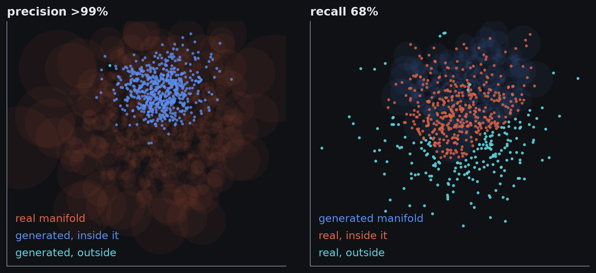
The guided diffusion model at its highest strength, measured against real examples of the class it was asked for. Left: nearly every generated sample lies inside the real data’s manifold. Right: a large share of the real examples lies outside the generated samples’ manifold.

• The samples are those of the guidance figure’s third panel.
• PROMPT: what would mode collapse score? Precision high, recall near zero.

Precision and recall: readings

Guidance strength	Precision	Recall
0	97%	96%
1	99%	97%
4	>99%	68%

• High precision, low recall: realistic but narrow
  • strong guidance, tight truncation, a low temperature, mode collapse
• High recall, low precision: varied but flawed
  • a high temperature
• Precision measures quality; recall measures diversity.

• The table is computed from the same samples as the two figures.
• Precision has little room to move here, because the unguided samples are already realistic. Recall is where the cost shows.
• Precision and recall measure the trade temperature introduced.

Comparing the families

The pairing problem: four answers

Family	Who supplies the pairing	Trained to	Pays with
GAN	nobody: a discriminator learns to tell the two sets apart	fool the discriminator	no probability, unstable training, coverage
Flow	the invertible map itself	maximise the exact likelihood	a restricted architecture
VAE	a learned encoder	maximise a bound on the likelihood	a bound and blur
Diffusion	a fixed noising process	predict the noise that was added	many sampling steps

• Nothing says which noise becomes which example. Each family is one way round that.

• PROMPT: cover the middle columns and ask the room to rebuild them from the family names.
• This table and the next are the revision objects for the generative half.

Properties of the families

	Efficient sampling	Sample quality	Coverage	Well-behaved latent	Disentangled latent	Efficient likelihood
GANs	✓	✓	✗	✓	?	n/a
VAEs	✓	✗	?	✓	?	✗
Flows	✓	✗	?	✓	?	✓
Diffusion	✗	✓	?	✗	✗	✗
Autoregressive	✗	✓	?	n/a	n/a	✓

• First four rows: the assignments Prince gives, which he calls disputable (Prince 2023)
• Last row: ours, for last session’s decoder
  • one pass per token, an exact likelihood by the chain rule, and no latent space

• No row is all ticks. That is the point of the table.
• A question mark means undecided in the field, not unknown to us alone.
• The autoregressive row’s quality tick is this course’s judgement about text.
• SOURCE: Prince figure 14.3.

Choosing a family

• TRY: for each brief, name a family and the property that decided it
  1. flag anomalous readings from a sensor
  2. generate product images from a text description
  3. let a user compress a face, then edit it interactively
• Anomalies: a flow; the exact probability of a new example is the output wanted
• Text to image: a guided diffusion model; sample quality, with seconds per image as the cost
• Interactive editing: a variational autoencoder; an encoder and a well-behaved latent space, with one fast pass each way
• Only one of the three was decided by sample quality

• LISTEN FOR: choosing by sample quality every time. Ask what the output of the system is: a number, an image, or an edit.
• Defensible alternatives: a VAE’s bound for anomalies; a GAN for editing, at the cost of having no encoder.
• This slide closes the generative survey. It is a natural stopping point.

Reinforcement learning

The reinforcement learning problem

• Until now: every model learned from a dataset somebody had collected
• Now: the only data are the consequences of the model’s own actions; the only feedback is a number that may arrive much later

Definition 17 Reinforcement learning is a framework for sequential decision-making in which an agent learns to choose actions in an environment so as to maximise the rewards it receives.

• Missing, against supervised learning
  • a target for every input: nobody says which action was right
  • feedback at once: a reward can come long after the action that earned it, the credit assignment problem
  • a fixed dataset: what the agent does decides what it sees next
• Also: the environment is random, so a good action can turn out badly

• This third stands alone. If it opens the second slot, nothing from the generative survey is needed except the temperature formula, late on.
• The standard illustration is chess: one reward at the end of the game, and the decisive move thirty moves earlier.
• SOURCE: Prince, opening of chapter 19.

A gridworld

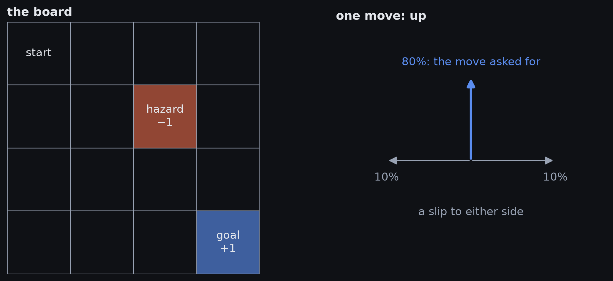
The running example. An agent moves on a grid; the goal pays +1, the hazard pays −1, and either ends the episode. A move goes where it was aimed most of the time and slips sideways otherwise.

• After Prince’s penguin on the ice, section 19.1.
• PROMPT: try to make this supervised. What is the target for “move right” in the start cell? There is none; let the room find that out.
• A move into the wall leaves the agent where it is.

Agent and environment

• The loop: the agent sees a state and takes an action; the environment returns a reward and the next state
• State \(s_t\): the situation the environment is in; here, the cell the agent occupies, which it sees in full
• Action \(a_t\): what the agent chooses; here, one of 4 moves
• Reward \(r_{t+1}\): one number from the environment after each action
• Episode: one run of the loop from a start to an end
• Elsewhere
  • a game: the character’s moves, and the score
  • a robot: its movements, and whether the task was done
  • a trader: buying and selling, and the profit
• Not a label: a reward says how good the outcome was, not which action would have been right

• SOURCE: Prince, opening of chapter 19, for the three examples.
• LISTEN FOR: “the reward is the loss”. A loss compares an output with a known target; a reward is all the agent ever gets.

Agent and environment: the loop

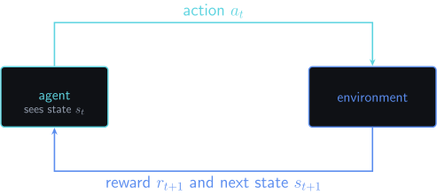
The agent chooses an action from the state it sees. The environment answers with a reward and a new state, and the loop repeats until the episode ends.

• After Prince figure 19.6.
• An episode is one run of the loop from a start to an end: one game, one walk across the grid.

The Markov decision process

Definition 18 A Markov decision process (MDP) consists of a set of states, a set of actions, transition probabilities \(\prob{s_{t+1}\mid s_t,a_t}\) and a reward distribution \(\prob{r_{t+1}\mid s_t,a_t}\). The next state and reward depend only on the current state and action, not on the history before them.

• On the grid: 16 states, 4 actions, the slip probabilities, and the two paying cells
• The Markov property: the present state is all the agent needs; how it got here adds nothing
• Why it matters: a state’s worth can be worked out one step at a time
• State against observation: an agent that sees only part of the state loses the property
  • one frame of a video game doesn’t show which way anything is moving

• The Markov property is a property of the problem as described to the agent, not of the agent.
• The video-game example comes back with deep Q-networks, which stack four frames to repair it.
• SOURCE: Prince section 19.1.

Return

Definition 19 The return \(\ret_t\) is the discounted sum of the rewards received after time \(t\), where the discount factor \(\discount\in(0,1]\) weights a reward \(k\) steps further into the future by \(\discount^{k}\).

\[ \ret_t=\sum_{k=0}^{\infty}\discount^{k}\,r_{t+k+1} \tag{7}\]

• Read aloud: the sum of future rewards, each one discounted once more for every step it is away
• Discount: near zero is short-sighted, near one is patient; on the grid \(\discount=0.9\)
• Worked: with no slips, 6 moves take the agent from the start to the goal, which then pays
  • \(\ret_0=0.9^{6}\times 1=0.53\)
• Reward against return: a reward is one step’s number; the return is the whole future’s

• EMPHASIS: the agent is not maximising the next reward. Every reward on the worked path but the last is zero.
• PROMPT: what would a discount of exactly one do to the agent’s hurry? Nothing would make a short path better than a long one.
• SOURCE: Prince equation 19.1.

Policy

Definition 20 A policy \(\policy(a\mid s)\) gives, for each state \(s\), a probability distribution over the actions \(a\). A deterministic policy puts all of that probability on one action.

• In plain terms: the agent’s behaviour, what it does in each situation
• Deterministic: one arrow in each cell of the grid
• Stochastic: a distribution over the four moves in each cell
  • a distribution over a small vocabulary of actions, like a next-token distribution over tokens
• The goal is the policy with the highest expected return.

• Everything after this slide is a way of finding that policy.
• The comparison with a language model is deliberate; it returns at the decision transformer.

Values

State values

• The return is known only when the episode is over. How good is the situation the agent is in now?

Definition 21 The state value \(\statevalue{s}\) is the expected return from starting in state \(s\) and following the policy \(\policy\) thereafter: \(\statevalue{s}=\expectsub{\policy}{\ret_t\mid s_t=s}\).

• In plain terms: the return to expect from here, on average, behaving this way
• The average is over: the policy’s random choices and the environment’s slips
• It depends on the policy: the same cell is worth more to an agent that plays well from it
• Notation: \(\statevalue{s}\) here and in Sutton and Barto (Sutton and Barto 2018); Prince writes \(v[s\mid\policy]\)

• LISTEN FOR: “the value of a cell is its reward”. On the grid most cells pay nothing, yet are worth something.
• SOURCE: Prince equation 19.2.

Action values

Definition 22 The action value \(\actionvalue{s}{a}\) is the expected return from starting in state \(s\), taking action \(a\), and following the policy \(\policy\) thereafter: \(\actionvalue{s}{a}=\expectsub{\policy}{\ret_t\mid s_t=s,\,a_t=a}\).

• One number per state and action: 16 cells by 4 moves on the grid
• Why it is the useful one: the best move is the largest action value; picking it needs no model of the environment
• Credit assignment: through the action value, a reward that arrives later is tied back to the action taken now
• Against the state value: the state value averages the action values over the policy’s choices
  • \(\statevalue{s}=\sum_{a}\policy(a\mid s)\,\actionvalue{s}{a}\)
  • under the best policy the average becomes a maximum: a state’s value is its largest action value

• These are the Q-values of Q-learning; the letter is all the name means.
• SOURCE: Prince equation 19.3, and equation 19.7 for the relation between the two.

Values on the grid

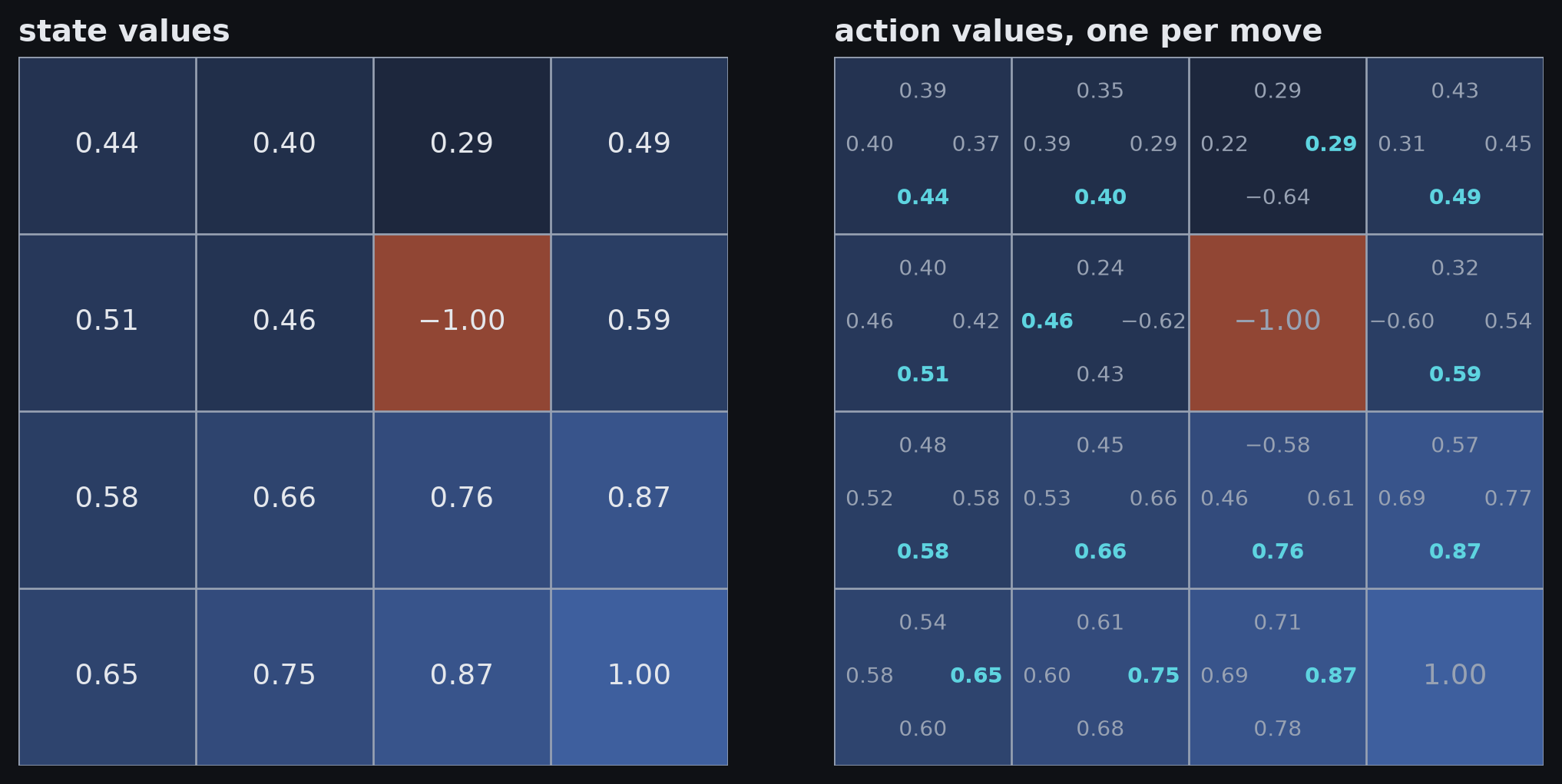
The grid’s values under its best policy. Left: one state value per cell. Right: the four action values of each cell, each written on the side its move aims at, with the largest highlighted.

• Computed exactly from the rules of the grid, with nothing learned.
• PROMPT: the cell above the hazard has one action value well below zero. Which, and why is it not minus one? The move can slip, and the reward is a step away.
• PROMPT: read the best policy off the right-hand panel. It goes down the left side and along the bottom, away from the hazard.
• After Prince figure 19.7.

The Bellman recursion

\[ \actionvalue{s}{a} = r(s,a) + \discount\sum_{s'}\prob{s'\mid s,a}\,\statevalue{s'} \tag{8}\]

• Read aloud: the value of an action is the reward it earns now, plus the discounted value of wherever it lands, averaged over where it might land
• Worked: third row, third column, moving down; the reward is zero there
  • \(0.9\times\bigl(0.8\times0.87+0.1\times0.87+0.1\times0.66\bigr)=0.76\), the highlighted number in that cell
• Consistency: the values of neighbouring states constrain one another
• Consequence: a value can be improved from its neighbours’ values, without waiting for the episode to end
• Scope: \(r(s,a)\) is written as one number because the grid’s reward is fixed; the definition of an MDP allows a distribution

• EMPHASIS: “now equals reward plus discounted next” is the idea every method in the next two sections is built on.
• The three terms in the bracket are the three places the move can land: straight on and a slip to each side.
• SOURCE: Prince equation 19.8.

Tabular methods

Estimating values

• The grid’s values were computed from its rules, but an agent dropped into a world doesn’t have the transition probabilities

Method	Needs the rules?	Learns from	Updates
Dynamic programming	yes	the rules alone	at any time
Monte Carlo	no	whole episodes	when an episode ends
Temporal difference	no	single steps and its own estimates	after every step

• Bootstrapping: updating an estimate from other estimates
• Temporal difference combines the other two: it samples like Monte Carlo and bootstraps like dynamic programming

• The values on the grid two slides back were dynamic programming: the rules were known.
• LISTEN FOR: “bootstrapping from guesses can’t work”. The reward in each step is real, and it drags the guesses towards the truth.
• SOURCE: Prince section 19.3.

Q-learning

• The table: one estimate \(q(s,a)\) for every state and action, all starting at zero
• After each step, one entry is moved

\[ q(s_t,a_t) \leftarrow q(s_t,a_t) + \alpha\Bigl( r(s_t,a_t)+\discount\max_{a}q(s_{t+1},a)-q(s_t,a_t) \Bigr) \tag{9}\]

• Read aloud: move the old estimate a little towards the reward plus the discounted best estimate at the next state
• The max: under the best policy a state’s value is its largest action value; here, the next state’s
• The bracket: a surprise, how much better or worse the step went than the table expected
• Week 2: old value plus a learning rate \(\alpha\) times an error, the shape of a gradient step
• Worked, with \(\alpha=0.1\): \(0.62+0.1\times\bigl(0+0.9\times0.86-0.62\bigr)=0.64\)

• The worked update is the same cell and move as the Bellman example, part-way through learning, landing in the cell below.
• The target inside the bracket is the Bellman recursion with one sampled landing place instead of the average over all of them.
• DO NOT introduce SARSA or the on-policy, off-policy distinction.
• SOURCE: Prince equation 19.15; the algorithm is from (Watkins and Dayan 1992).

Q-learning on the grid

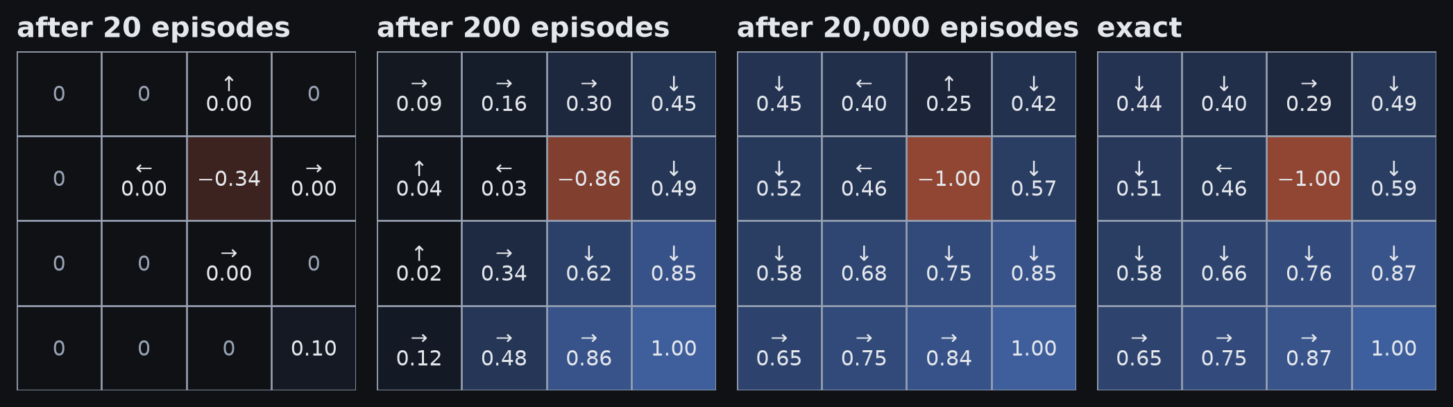
The table as it is learned. Each cell shows its largest action value and the move that has it; the last panel is the exact answer from the rules. Value spreads backwards from the two paying cells.

• The agent was never given the slip probabilities or the rewards. It found the values by acting.
• PROMPT: in the first panel, why are the cells far from the goal still zero? No reward has reached them yet.
• The learned values still wobble at the end: the learning rate is constant and the world is random. Two top-row arrows differ from the exact panel; those moves are near-ties.

Exploration against exploitation

• An agent that always takes its current best action never learns whether another was better
• An agent that always acts at random never uses what it has learned
• Supervised learning never had this problem: its data didn’t depend on its guesses

Definition 23 An epsilon-greedy policy takes a uniformly random action with probability \(\epsilon\), and otherwise takes the action with the highest estimated action value.

• On the grid: the table in the last figure was learned with \(\epsilon=0.2\)
• Limitation: when it explores, the worst action is as likely as the second best

• PROMPT: with epsilon at zero from the start, what does the first panel of the last figure look like for ever? The agent repeats the first thing that didn’t hurt.
• This epsilon is a probability, not diffusion’s noise symbol.
• SOURCE: Prince section 19.3.

Softmax policies

\[ \policy(a\mid s) = \frac{\exp\!\left(q(s,a)/\tau\right)}{\sum_{a'}\exp\!\left(q(s,a')/\tau\right)} \tag{10}\]

• Boltzmann policy: the softmax with temperature, Equation 1, with action values in place of logits
• High \(\tau\): close to uniform; the agent explores
• Low \(\tau\): nearly all the probability on the best action; the agent exploits
• One cell of the grid, its best move against its worst
  • at \(\tau=1\): 35% against 9%
  • at \(\tau=0.05\): 95% against <1%
• Unlike epsilon-greedy: better actions are tried more often than worse ones
• One formula sets how varied a language model’s text is and how much an agent explores.

• The temperature formula’s last appearance. Here it acts during learning, and the trade is exploitation against exploration.
• A common schedule: start hot and cool down as the estimates improve.
• SOURCE: Prince problem 19.4, equation 19.45.

Deep reinforcement learning

Deep Q-networks

• A table has one row per state, but a screen of pixels has far too many states for one

Definition 24 A deep Q-network replaces the table of action values with a network that takes a state and outputs one action value for each action.

• Why a network: it generalises, so a screen never seen before gets values like those of similar screens
• Input: the last four frames of the game, through week 4’s convolutional layers
• Loss: the Q-learning surprise, squared
• Result: one architecture, trained separately on each of 49 Atari games, at about the level of a professional game tester overall (Mnih et al. 2015)
  • above human level on some games, but almost no progress on others
• What it took: experience replay, training on stored past steps; and a target network, a copy updated only now and then

• Four frames, because one frame doesn’t show velocity: the Markov property, repaired by redefining the state.
• The game with almost no progress was Montezuma’s Revenge: rewards too sparse for random exploration to find.
• The cost: around 38 days of game experience per game.
• SOURCE: Prince section 19.4.

Policy gradients

• Must the agent learn values at all?

Definition 25 A policy gradient method learns a stochastic policy directly: a network with trainable parameters maps a state to a distribution over actions, and those parameters are adjusted to make actions that led to high return more probable.

• Training, in words: play episodes with the current policy; raise the probability of the actions taken in episodes that went well
• Why choose it
  • continuous actions: no table, so no largest entry to pick
  • partly observed tasks: when two states look alike, a random choice can be the best one
  • exploration comes built in, since the policy is a distribution
• The cost: noisy updates, because whole episodes are judged at once
• Name: the basic algorithm is REINFORCE (Williams 1992)

• No equation by design. DO NOT derive the policy gradient.
• The policy network’s output layer is a softmax over actions: the same head as a classifier or a language model.
• SOURCE: Prince section 19.5, whose reasons are exploration, a loss that changes smoothly, and partial observability; continuous actions is our addition.

Actor and critic

Definition 26 An actor-critic method trains two networks together: the actor is the policy, and the critic estimates state values, which stand in for the future rewards the actor would otherwise have to wait for.

• Actor: the policy network, which chooses the actions
• Critic: a value network, which judges the state each action led to
• What the critic buys: the actor is updated after every step, with no wait for the episode to end
• An actor-critic method is a policy gradient with temporal-difference updates
• Compare: two networks trained on each other’s outputs, as in a GAN, but here they cooperate

• SOURCE: Prince section 19.6.

The decision transformer

• Offline: learn from logged episodes without ever acting in the environment
  • for when exploring is dangerous or expensive

Definition 27 The decision transformer treats offline reinforcement learning as sequence modelling: a transformer decoder reads returns-to-go, states and actions as tokens and predicts the next action.

• Return-to-go: the total reward still to come from this point in the logged episode
• Training: last session’s next-token prediction, on the action tokens
• Acting: ask for a high return and generate the action that goes with it
• The return asked for is a condition, like a class label or a prompt.
• Not imitation: imitation copies the logged agent whatever it earned; here the return asked for selects the behaviour

• This is where the two halves of the session meet: the return-to-go is a condition, exactly like a class label or a prompt.
• During acting, the return asked for is reduced by each reward received.
• SOURCE: Prince section 19.7, figure 19.17; the paper is (Chen et al. 2021).

Episodes as sequences

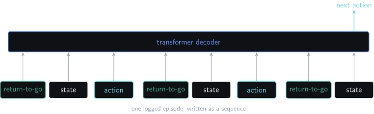
The decision transformer’s input. A logged episode is written as return-to-go, state, action, repeated; the decoder predicts the action that follows the latest state.

• After Prince figure 19.17.
• PROMPT: what plays the part of the prompt here? The return-to-go.

Methods compared

Learns	Methods	Gives up
values, from known rules	dynamic programming	any world whose rules aren’t given
values, from experience, in a table	Monte Carlo, temporal difference, Q-learning	large state spaces
values, with a network	deep Q-networks	stable training: the target moves as the network learns
the policy	policy gradients	low-noise updates
both	actor-critic	simplicity: two networks to balance
from logs alone	decision transformer	the chance to explore

• Each row answers a limit of the row above.

• PROMPT: for each row, what limit of the row above does it answer? Unknown rules; too many states; no need for values, and continuous actions; noisy whole-episode updates; not being allowed to act.
• This table is the revision object for the reinforcement-learning third.

Revision

Quality and diversity controls

Where	The knob	For typical, similar outputs	For varied outputs
a language model’s sampler	temperature on the logits	low	high
a GAN	truncation threshold on the latent	tight	loose
a diffusion model	guidance strength	strong	weak
an agent’s policy	temperature on the action values	low: exploit	high: explore

• Each knob trades typical outputs against varied ones.
• First three rows: applied after training; precision measures the quality and recall the diversity
• Last row: the first row’s formula, applied while the agent learns

• PROMPT: cover the last two columns. For each row, which way is “safe”?
• The first and last rows are the same formula, Equation 1 and Equation 10.

Generative and probabilistic generative

• TRY: GAN, flow, VAE, diffusion model, last session’s decoder. Which can assign a probability to an example?
• All but the GAN
  • exactly: the flow and the decoder
  • as a lower bound: the VAE and the diffusion model
• What a probability allows
  • training by maximum likelihood
  • comparing two models on held-out data
  • flagging an example as an outlier
• What the GAN has instead: a discriminator, during training only

• LISTEN FOR: “generative means probabilistic”. The GAN is the counterexample. Definition 2 does not mention probability.

Training signals

• TRY: for each family, what is the network asked to get right on one training step?
• GAN: the discriminator, to tell real from generated; the generator, to make it fail
• Flow: to make the training example probable, exactly
• VAE: to rebuild the example from the encoder’s latents, while keeping those latents near the prior
• Diffusion: to name the noise that was added
• The question all four answer: nothing says which noise becomes which example

• If one row is shaky, go back to that family’s trade-offs slide and to “The pairing problem: four answers”.

Reward, return and value

• TRY: for the start cell of the grid, give a reward, a return and a value
• Reward: one step’s number; acting from the start cell pays 0
• Return: the discounted sum over one episode that happened; the worked path’s was 0.53
• Value: the expected return over everything that could happen; 0.44 under the best policy
• Why is the value lower than the worked return?
• The worked path had no slips; the value averages over paths that do

• A return is one sample; a value is the average of such samples.
• LISTEN FOR: “the start cell’s value is zero because its reward is zero”.

Equations to recognise

• Softmax with temperature, Equation 1: divide the logits by \(\tau\), then take the softmax
• Flow density, Equation 4: the base density at the latent, divided by the map’s stretch
• Evidence lower bound, Equation 5: how well the example is rebuilt, minus the distance from the prior
• Noise prediction, Equation 6: squared error between the noise predicted and the noise added
• Return, Equation 7: future rewards, discounted and summed
• Bellman recursion, Equation 8: reward now, plus the discounted value of where the action lands
• Q-learning, Equation 9: move an estimate towards the reward plus the discounted best next estimate
• For each: say it aloud and name every symbol in it

• Recognition and reading, in line with how the session treated them: stated, read, and none derived.

Reading

Sources for this session

• Chapter 14, “Unsupervised learning”, in Prince, Understanding Deep Learning (Prince 2023): all of it
• Chapters 15 to 19: start with the opening section of each
  • the slides also draw on truncation and conditional GANs, the evidence lower bound and reparameterisation, the diffusion loss and guidance, and the tabular, deep Q-network and decision transformer sections
• Temperature: section 2 of Hinton et al. (Hinton et al. 2015)
• Reinforcement learning, further: Sutton and Barto, whose notation today’s slides use (Sutton and Barto 2018)
• Notebooks, as on this week’s lab card: the GAN toy example, one-dimensional flows, latent variable models, the diffusion encoder, dynamic programming and temporal difference methods
• Original papers: cited on the slides, listed on the next

References

Brock, Andrew, Jeff Donahue, and Karen Simonyan. 2018. Large Scale GAN Training for High Fidelity Natural Image Synthesis. https://arxiv.org/abs/1809.11096.

Chen, Lili, Kevin Lu, Aravind Rajeswaran, et al. 2021. Decision Transformer: Reinforcement Learning via Sequence Modeling. https://arxiv.org/abs/2106.01345.

Goodfellow, Ian J., Jean Pouget-Abadie, Mehdi Mirza, et al. 2014. Generative Adversarial Networks. https://arxiv.org/abs/1406.2661.

Heusel, Martin, Hubert Ramsauer, Thomas Unterthiner, Bernhard Nessler, and Sepp Hochreiter. 2017. GANs Trained by a Two Time-Scale Update Rule Converge to a Local Nash Equilibrium. https://arxiv.org/abs/1706.08500.

Hinton, Geoffrey, Oriol Vinyals, and Jeff Dean. 2015. Distilling the Knowledge in a Neural Network. https://arxiv.org/abs/1503.02531.

Ho, Jonathan, Ajay Jain, and Pieter Abbeel. 2020. Denoising Diffusion Probabilistic Models. https://arxiv.org/abs/2006.11239.

Ho, Jonathan, and Tim Salimans. 2022. Classifier-Free Diffusion Guidance. https://arxiv.org/abs/2207.12598.

Kingma, Diederik P, and Max Welling. 2013. Auto-Encoding Variational Bayes. https://arxiv.org/abs/1312.6114.

Kynkäänniemi, Tuomas, Tero Karras, Samuli Laine, Jaakko Lehtinen, and Timo Aila. 2019. Improved Precision and Recall Metric for Assessing Generative Models. https://arxiv.org/abs/1904.06991.

Mnih, Volodymyr, Koray Kavukcuoglu, David Silver, et al. 2015. “Human-Level Control Through Deep Reinforcement Learning.” Nature 518 (7540): 529–33. https://doi.org/10.1038/nature14236.

Prince, Simon J. D. 2023. Understanding Deep Learning. MIT Press. https://udlbook.github.io/udlbook/.

Rezende, Danilo Jimenez, and Shakir Mohamed. 2015. Variational Inference with Normalizing Flows. https://arxiv.org/abs/1505.05770.

Sohl-Dickstein, Jascha, Eric A. Weiss, Niru Maheswaranathan, and Surya Ganguli. 2015. Deep Unsupervised Learning Using Nonequilibrium Thermodynamics. https://arxiv.org/abs/1503.03585.

Sutton, Richard S., and Andrew G. Barto. 2018. Reinforcement Learning: An Introduction. 2nd ed. MIT Press. http://incompleteideas.net/book/the-book-2nd.html.

Watkins, Christopher J. C. H., and Peter Dayan. 1992. “Q-Learning.” Machine Learning 8 (3-4): 279–92. https://doi.org/10.1007/bf00992698.

Williams, Ronald J. 1992. “Simple Statistical Gradient-Following Algorithms for Connectionist Reinforcement Learning.” Machine Learning 8 (3-4): 229–56. https://doi.org/10.1007/bf00992696.