Lecture 10: Transformers

Week 5 · architectures

Eoin O’Brien

The sequence modelling problem

Text as a sequence

• Images arrive on a regular grid; text arrives as a sequence of tokens
• Token: one discrete unit produced by a tokenizer, often a word fragment and not a whole word
• Sequence length varies from one example to the next
• Each token will become a vector, so even a short passage is a long input
• A fully connected layer over the whole sequence would
  • require a fixed input length
  • learn different parameters for different positions
  • scale poorly as the sequence grows
• We want one set of parameters that can process many positions and many sequence lengths.

One vector per position

• For a sequence of \(N\) token positions, \(\vect{x}_n\in\reals^{D}\) is the current vector representation at position \(n\)
• Read: “x n”, the \(n\)th of \(N\) vectors, each with \(D\) entries
• One position, one vector
• \(\vect{x}_n\) is whatever representation the model holds at position \(n\)
  • building the first one from a token is a separate step, later today
• A sequence model works on one vector per position, not on token IDs or strings.

Token vectors

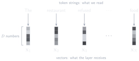
The model receives the text as an ordered sequence of vectors, one D-dimensional vector per position.

Position and relevance

The restaurant refused to serve me a ham sandwich because it only cooks vegetarian food.

• TRY: which word does it refer to, and which words told you?
• Interpreting it requires information from restaurant
• “Look at the previous word” fails, and so does “look at the nearest noun”
• Relevant words may be nearby or far apart
• Which positions matter depends on the content of the sequence.
• So a sequence model needs data-dependent connections between positions

PROMPT: take answers to the TRY before revealing. Then ask: what would change if every position could directly inspect every other position?

A long-range reference

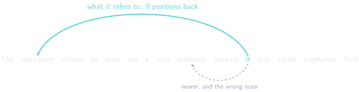
it refers to restaurant, far to its left, not to the nearer noun sandwich.

A fixed-weight sum

• Week 4’s convolution builds each output from the positions around it

\[ z_n=\sum_{j=1}^{3}\omega_j\,x_{n+j-2} \]

• Read: “z n is a weighted sum of x n and its two neighbours”; week 4’s \(z_i\), with one number per position
• The weights: one per offset, learned once, the same for every input
• it needs restaurant, 9 positions back in this sentence
  • the next sentence puts the word it needs at a different offset
• A wider kernel reaches further, but still gives each offset one fixed weight
• We want weights computed from the sequence itself.

Attention as a weighted average

A weighted average at one position

The restaurant refused to serve me a ham sandwich because it only cooks vegetarian food.

• We are updating the vector at it
• The idea: replace that vector with a weighted average of the vectors at every position, its own included

\[ \vect{y}_{\text{it}} =0.61\,\vect{x}_{\text{restaurant}} +0.08\,\vect{x}_{\text{it}} +0.06\,\vect{x}_{\text{sandwich}} +\cdots \]

• \(\vect{y}_{\text{it}}\): the new vector at it; an output, not week 1’s target
• Weights: none negative, and summing to one over the 15 positions, one token per word here; the numbers are illustrative
• What it buys: the vector at it now carries information from restaurant, which later layers need to make sense of cooks
• Against a convolution: these weights are shares of one whole, and were chosen for this sentence by what its tokens are

The weights at one position

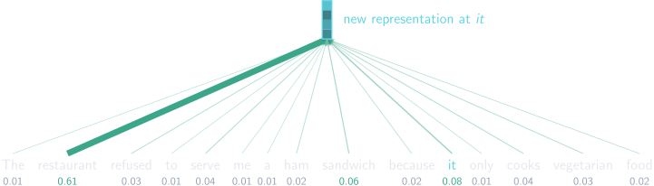
Every token contributes to the new vector at it. Line width shows how much. The weights are illustrative; they sum to one.

A first version: mixing the token vectors

• The same average, for any position \(n\)

\[ \vect{y}_n=\sum_{m=1}^{N}a_{mn}\vect{x}_m \tag{1}\]

• Read: “y n is the sum over sources of weight times vector”
• Source \(m\) contributes; destination \(n\) receives
• \(a_{mn}\): the share of source \(m\) in the new vector at destination \(n\)
• Two things are still missing
  • where the weights come from
  • whether all of \(\vect{x}_m\) should be passed on, or only part of it

Attention weights

Definition 1 The attention weight \(a_{mn}\) is the weight that source position \(m\)’s contribution gets in the mixture forming the new representation at destination position \(n\). For each destination \(n\), the weights are non-negative and sum to one over the sources \(m\).

\[ a_{mn}\ge 0, \qquad \sum_{m=1}^{N}a_{mn}=1 \tag{2}\]

• Read: “a m n”, how much source \(m\) contributes to destination \(n\)
• Index order: source first, destination second, in every equation today
• In Prince: \(a[\vect{x}_m,\vect{x}_n]\)
• In the sentence: \(a_{2,11}=0.61\), the share of restaurant, position 2, in the new vector at it, position 11
  • \(a_{11,2}\) is a different number: the share of it in the new vector at restaurant
• Each destination gets its own distribution of weights

Choosing the weights: a first try

• The weights should come from the sequence itself
• Rule: score source \(m\) for destination \(n\) by \(\inner{\vect{x}_m}{\vect{x}_n}\); a larger score gets a larger weight
• Week 1: multiply matching entries and add; large when the two vectors point the same way
• Suppose every token vector has the same length
• TRY: which source scores highest for it? Compare the score of restaurant for it with the score of it for restaurant

PROMPT: take both halves of the TRY before moving on. “Restaurant” is the common first answer; ask what the dot product of a vector with itself is.

• Itself: \(\inner{\vect{x}_n}{\vect{x}_n}\) is the largest score, so the new vector at it is mostly the old one
• Symmetric: \(\inner{\vect{x}_m}{\vect{x}_n}=\inner{\vect{x}_n}{\vect{x}_m}\)
  • the score can’t say that it needs restaurant more than restaurant needs it
• Alignment: a high score needs two vectors that point the same way, but nothing makes the vectors of it and restaurant do so
• What a position asks for and what it is found by need different vectors.

A soft dictionary lookup

• A Python dict holds keys and values: d[query] returns the one value whose key equals the query
• Attention is the same lookup, made soft
  • the query is compared with every key; each match is a matter of degree
  • the result is a blend of all the values, weighted by how well each key matched
• Query: what the lookup asks for
• Key: what an entry is found by
• Value: what the entry hands over; it need not resemble the key
• Attention separates matching information from transferred information.
• Limit of the analogy: queries, keys and values are computed from each sequence by learned maps; nothing is stored

Three roles

	it	restaurant	sandwich
Query: what it asks for	a noun that can act	…	…
Key: what it is found by	a pronoun, a subject	a noun that can act	a noun that can’t
Value: what it hands over	…	a place that serves food	a food

• Key and value differ: what makes restaurant findable is not what is worth copying
• Query and key differ: it asks for one thing, and is found by another when cooks looks for its subject
• Every token has all three; the gaps are the ones this example doesn’t use
• Status: glosses for this example; learned features carry no labels

The three projections

Definition 2 Each position \(m\) turns its representation \(\vect{x}_m\) into three vectors by three learned affine maps: a query \(\vect{q}_m\), used when the position asks for information; a key \(\vect{k}_m\), used when it is matched as a source; and a value \(\vect{v}_m\), the payload it can contribute.

\[ \vect{q}_m=\layerbias_q+\layerweights_q\vect{x}_m, \qquad \vect{k}_m=\layerbias_k+\layerweights_k\vect{x}_m, \qquad \vect{v}_m=\layerbias_v+\layerweights_v\vect{x}_m \tag{3}\]

• Read: “q m is beta q plus Omega q times x m”: a matrix product plus a bias
• Shapes: \(\vect{q}_m,\vect{k}_m\in\reals^{D_q}\) and \(\vect{v}_m\in\reals^{D_v}\), so \(\layerweights_q,\layerweights_k\) are \(D_q\times D\) and \(\layerweights_v\) is \(D_v\times D\)
• Shared dimension: a query is compared with a key entry by entry, so both have \(D_q\) entries
• Shared parameters: the same three maps at every position
• Projection: this deck’s name for one of these maps; each entry of a key is a learned weighted sum of the entries of \(\vect{x}_m\), and the three maps learn different sums

Query, key and value

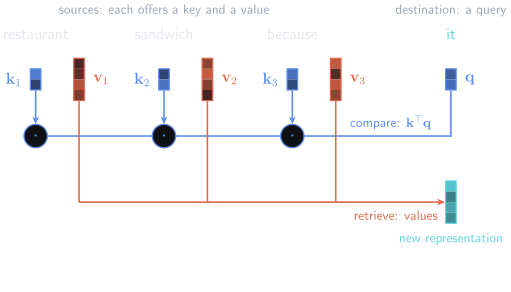
The position being updated emits a query. Each source offers a key to match against and a value to retrieve.

The score

Definition 3 The score \(s_{mn}\) of source position \(m\) for destination position \(n\) is the dot product of key \(m\) with query \(n\).

\[ s_{mn} =\inner{\vect{k}_m}{\vect{q}_n} =\sum_{j=1}^{D_q}k_{mj}\,q_{nj} \tag{4}\]

• Read: “s m n”, key \(m\) dotted with query \(n\): one scalar per pair
• The dot product from week 1: multiply matching entries and add
  • positive when the two vectors align; larger in size when either is longer
• Range: any real number, negative included

The score: compatibility

• Compatibility, not similarity: the projections learn which features and scales matter for matching
  • a high score says this key suits this query; the two tokens need not mean similar things
  • Prince calls the dot product a measure of similarity; the vectors it compares are the projected key and query
• Not symmetric: \(s_{mn}\) uses key \(m\) and query \(n\); \(s_{nm}\) uses key \(n\) and query \(m\)
• No self-preference: \(s_{nn}=\inner{\vect{k}_n}{\vect{q}_n}\) compares two different vectors
• The first try’s three defects are gone

One score by hand

• A toy case with \(D_q=2\): the query at it and the key at restaurant
• Read the two entries as noun-like and can act: a gloss for this toy only

\[ \vect{q}_{\text{it}}=\begin{bmatrix}2\\1\end{bmatrix}, \qquad \vect{k}_{\text{restaurant}}=\begin{bmatrix}1.2\\0.8\end{bmatrix} \]

• Multiply matching entries and add: \(1.2\times2+0.8\times1=3.2\)
• TRY: the keys at sandwich and because are \([1.2,-1.6]\) and \([-0.1,-0.1]\). Score each against the same query
• sandwich: \(1.2\times2+(-1.6)\times1=0.8\)
• because: \((-0.1)\times2+(-0.1)\times1=-0.3\)
• restaurant has both features the query asks for, sandwich has one, because has neither
• The numbers are illustrative; a trained model’s queries and keys have many more entries

PROMPT: students compute both scores before the reveals. Watch for a dropped sign on the negative entries.

One query against every key

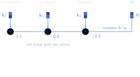
The query at it is scored against each source’s key. The scores are illustrative.

Learned scores

• The model receives no label saying that restaurant is the word it refers to
• Training shapes the projections so that useful query–key matches score highly
• Why three: the arithmetic stays visible; the real computation scores all \(N\) sources

Softmax over one query’s scores

• Scores are any real numbers; weights must be positive and sum to one
• Week 2’s softmax: there it turned logits into class probabilities; here it turns one query’s scores into shares over the sources

\[ a_{mn} =\softmax_m\!\left(s_{mn}\right) =\frac{\exp(s_{mn})}{\sum_{m'=1}^{N}\exp(s_{m'n})} \tag{5}\]

• Read: “the softmax over m”: exponentiate every score for query \(n\), then divide each by their total; \(m'\) runs over the sources in that total
• Positive: \(\exp\) of any real number is positive
• Sums to one over \(m\): each weight is a share of the same total
• Relative: only the gaps between scores matter; raising one score lowers every other weight for that query
• A score is not a weight: a score is any real number, a weight is one query’s share.

Softmax by hand

• The three scores for it: \([3.2,0.8,-0.3]\)
• Exponentiate: \([24.53,2.23,0.74]\)
• Add: \(27.50\)
• Divide: \([0.89,0.08,0.03]\)
• Normalisation set: over all 15 sources the same score gives restaurant \(0.61\), because the total is larger
• TRY: new scores, \([2,2,0]\). Before computing: which weights are equal, and is the third zero?
• \([0.47,0.47,0.06]\): equal scores take equal shares; no finite score gives a weight of zero

PROMPT: hands up for “the third weight is zero” before computing anything. It is the commonest wrong prediction and the reason the Positive bullet matters.

Scores to weights

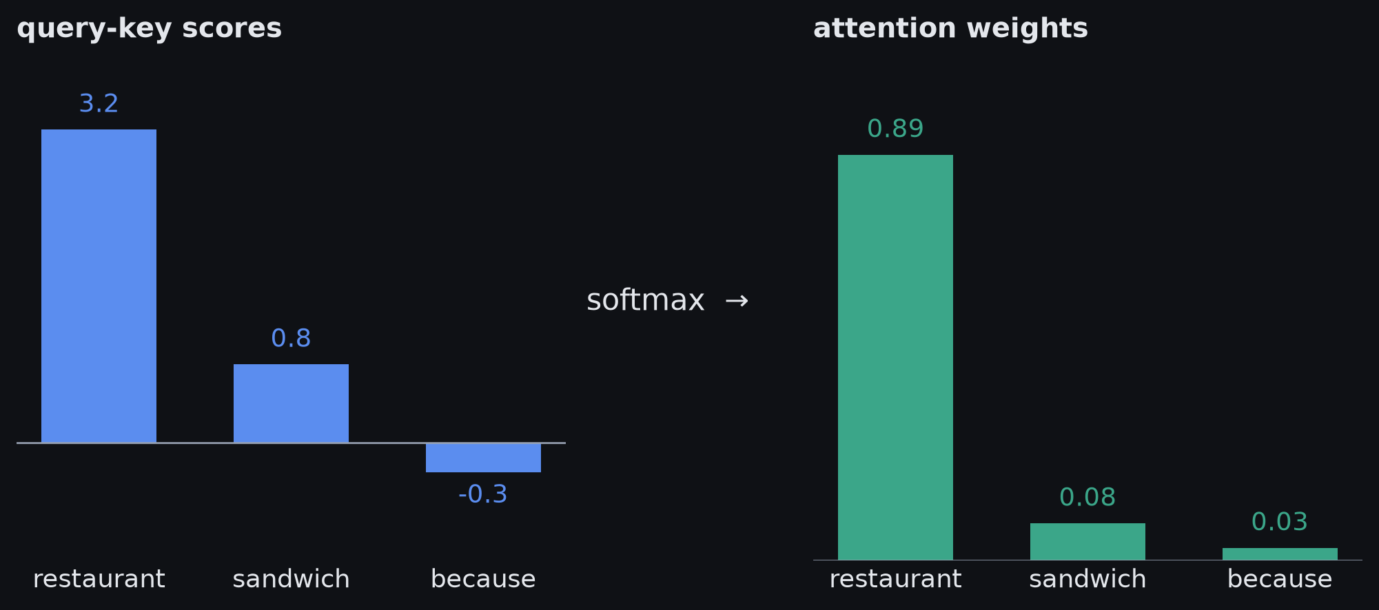
Scores can be negative and need not sum to one. Softmax turns them into positive weights that do.

The weighted average of values

• Once the weights are known, the queries and keys have done their job
• The first version mixed the token vectors, Equation 1; the finished one mixes the values

\[ \vect{y}_n=\sum_{m=1}^{N}a_{mn}\vect{v}_m \tag{6}\]

• Read: “y n is the sum over sources of weight times value”
• In Prince: \(\mathrm{sa}_n[\vect{x}_1,\ldots,\vect{x}_N]\)
• Shape: \(\vect{y}_n\in\reals^{D_v}\), the same as one value
• Why not \(\vect{x}_m\): it holds everything about the token; \(\layerweights_v\) selects what is worth passing on
• In the toy case: \(\vect{y}_{\text{it}}=0.89\,\vect{v}_{\text{restaurant}}+0.08\,\vect{v}_{\text{sandwich}}+0.03\,\vect{v}_{\text{because}}\)
• Different destinations mix the same values in different proportions: the weights route each value to where it is wanted
• Attention is learned, content-dependent information routing.

A weighted mixture of values

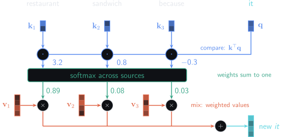
The query–key scores set the weights. The weights mix the value vectors into the output at the query’s position.

One output, end to end

1. Create the query \(\vect q_n\) at destination \(n\)
2. Create a key \(\vect k_m\) and a value \(\vect v_m\) at every source \(m\)
3. Score \(\vect q_n\) against every \(\vect k_m\)
4. Softmax the scores into weights \(a_{mn}\)
5. Mix the \(\vect v_m\) with those weights

\[ \vect{y}_n =\sum_{m=1}^{N} \softmax_m\!\left(\inner{\vect{k}_m}{\vect{q}_n}\right) \vect{v}_m \tag{7}\]

The equation comes last on purpose: it compresses the five steps and isn’t where they start.

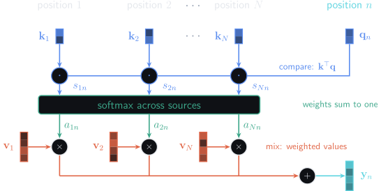
Query against keys gives scores, softmax gives weights, and the weights mix the values into the new representation.

Self-attention

• Nothing makes it a special destination
  • every token emits its own query and receives its own weighted mixture
• Every position plays two parts
  • destination, through its query
  • source, through its key and value

Definition 4 Self-attention computes Equation 7 at every position \(n\) of one sequence, with the queries, keys and values all derived from that same sequence.

Every position as a query

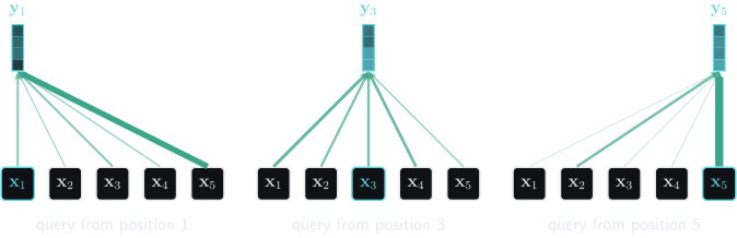
Three of the five queries over one small random sequence. The sources are the same; each query weights them differently.

Self-attention and nonlinearity

• With the weights held fixed, \(\vect{y}_n=\sum_m a_{mn}\vect{v}_m\) is linear in the values, and so affine in the inputs
• But the weights are functions of the input: \(a_{mn}=\softmax_m\!\left(\inner{\vect{k}_m}{\vect{q}_n}\right)\)
• TRY: set the biases to zero and double every input \(\vect{x}_m\). What happens to the values, and to the scores?
• The values double; a score multiplies two projections, so it quadruples
• Softmax depends on the gaps between scores, and those quadruple too
• So the weights change; doubling the input doesn’t double the output
• Changing the sequence changes which routes carry information: the whole operation is nonlinear.

Sequence length and parameters

• The same query, key and value projections are reused at all \(N\) positions
• The layer’s parameter count does not grow with sequence length
• The layer returns one output per input position
• So the same trained layer can process different values of \(N\)

All-to-all interactions

• Each of \(N\) queries is compared with \(N\) keys

\[ \text{number of attention scores}=N^2 \]

• Every output can directly take in every input value
• Benefit: short paths for long-range dependencies
• Cost: computation that grows with the square of the sequence length; the section on long sequences returns to it

The N by N interaction grid

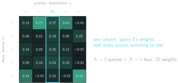
Every query is scored against every key, which is N² scores. Each column holds one query’s weights, for the same sequence.

Recurrence

• Before transformers, recurrent neural networks (RNNs) were the standard sequence model
• Hidden state \(\hidden_n\): one vector, a running summary of positions \(1,\ldots,n\)
• One learned transition \(f\) updates the summary with each new token

\[ \hidden_n = f\!\left(\hidden_{n-1},\vect{x}_n\right) \tag{8}\]

• Read: “h n is f of the previous summary and the current token”
• Shared parameters: the same \(f\) at every position
• Any length: apply \(f\) once per token

Recurrence: two limits

• Information from an early token reaches a later one only through every hidden state in between

\[ \hidden_1 \rightarrow \hidden_2 \rightarrow \cdots \rightarrow \hidden_n \]

• Long dependency paths: information that must travel far passes through many transitions
  • so do its gradients, with the same shrinking and growing as through many layers
• Limited parallelism: position \(n\) waits for the hidden state from position \(n-1\)
• LSTMs and GRUs add gates, learned switches on what the hidden state keeps and forgets
  • they train over longer spans; the step-by-step dependency remains

Path length: recurrence and attention

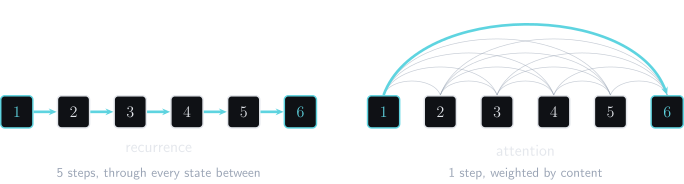
Recurrence passes information through every intermediate state. Attention connects two distant positions in one layer.

Matrix form

The token matrix

• The recipe so far is a double loop over \(n\) and \(m\); the matrix form is the same computation, vectorised
• Place the \(N\) token vectors in the columns of one matrix

\[ \mat{X}= \begin{bmatrix} \vert & & \vert\\ \vect{x}_1 & \cdots & \vect{x}_N\\ \vert & & \vert \end{bmatrix} \in\reals^{D\times N} \tag{9}\]

• Project every column at once

\[ \mat{Q}=\layerweights_q\mat{X},\qquad \mat{K}=\layerweights_k\mat{X},\qquad \mat{V}=\layerweights_v\mat{X} \tag{10}\]

• Shapes: \(\mat{Q}\) and \(\mat{K}\) are \(D_q\times N\); \(\mat{V}\) is \(D_v\times N\)
• Columns: column \(m\) of each is \(\vect{q}_m\), \(\vect{k}_m\) or \(\vect{v}_m\)
• Biases: left out to keep the line short; each \(\layerbias\) is added to every column

The score matrix

• One product holds all \(N^2\) scores

\[ \mat{S}=\mat{K}\transpose\mat{Q} \in\reals^{N\times N}, \qquad s_{mn}=\inner{\vect{k}_m}{\vect{q}_n} \tag{11}\]

• Shape: \((N\times D_q)(D_q\times N)\rightarrow N\times N\)
• Entry \((m,n)\): row \(m\) of \(\mat{K}\transpose\) is key \(m\); column \(n\) of \(\mat{Q}\) is query \(n\); their product is Equation 4
• Column \(n\): every key’s score for query \(n\)
• Row \(m\): key \(m\)’s score against every query
• TRY: which entry holds key 2 against query 3? What would \(\mat{Q}\transpose\mat{K}\) hold instead?
• \(s_{23}\); the other product puts queries in rows, the transpose of this matrix

One column of the score matrix

• The toy keys as the columns of \(\mat{K}\), and the query at it

\[ \mat{K}=\begin{bmatrix}1.2&1.2&-0.1\\0.8&-1.6&-0.1\end{bmatrix}, \qquad \vect{q}=\begin{bmatrix}2\\1\end{bmatrix} \]

• \(\mat{K}\transpose\vect{q}\) is that query’s column of \(\mat{S}\)

\[ \mat{K}\transpose\vect{q} =\begin{bmatrix}1.2&0.8\\1.2&-1.6\\-0.1&-0.1\end{bmatrix}\,\begin{bmatrix}2\\1\end{bmatrix} =\begin{bmatrix}3.2\\0.8\\-0.3\end{bmatrix} \]

• The same three scores as by hand, from one \((3\times 2)(2\times 1)\) product
• Softmax down the column: this query’s weights, \([0.89,0.08,0.03]\)
• Convention: tokens are columns here, as in Prince; many papers and libraries put tokens in rows, and the algebra transposes

Entries of the score matrix

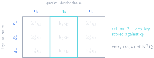
Entry (m,n) of KᵀQ is the dot product of key m and query n, so column n holds every score for query n.

Self-attention in matrix form

• Softmax each column of the scores to get the weight matrix \(\mat{A}\), with entries \(a_{mn}\)
• Then mix the value columns

\[ \operatorname{SA}(\mat{X}) = \mat{V}\mat{A} = \mat{V} \operatorname{Softmax}_{\text{columns}} \!\left(\mat{K}\transpose\mat{Q}\right) \tag{12}\]

• Read: “V times the column-wise softmax of K transpose Q”
• Shape flow: \((D_v\times N)(N\times N)\rightarrow D_v\times N\)
• Output column \(n\): a matrix times a column is a weighted sum of the matrix’s columns, so column \(n\) of \(\mat{V}\mat{A}\) is \(\sum_m a_{mn}\vect{v}_m\)
  • which is Equation 6
• In Prince: \(\mathrm{Sa}[\mat{X}]\), with square brackets

Order and representation

Token order

• TRY: swap two columns of \(\mat{X}\). What happens to the output columns?
• They swap, and nothing else changes
• Why: a score depends on which two vectors meet, not on where they sit
• So self-attention, as defined so far, permutes its outputs whenever its inputs are permuted
• The woman ate the raccoon and The raccoon ate the woman hold the same token vectors, rearranged
  • so the output at woman is the same vector in both: nothing reading it can tell who ate whom
• The layer needs a way to tell where each token occurs.

Permuting the tokens

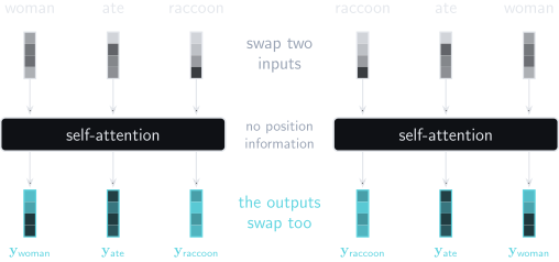
Without position information, reordering the inputs reorders the outputs and changes nothing else.

Positional encodings

Definition 5 A positional encoding is information about position supplied to the layer, so that it can tell positions apart.

• The simplest kind is one vector per position, added to the token at that position

\[ \mat{X}'=\mat{X}+\mat{\Pi} \tag{13}\]

• Read: “X prime is X plus Pi”
• Shape: \(\mat{\Pi}\) is \(D\times N\), the same as \(\mat{X}\); column \(n\) depends only on the position \(n\)
• Each position gets a distinct vector, fixed in advance or learned
  • learned: one more table of vectors, a column per position, trained like any other weights

• In the example: with \(\vect{\pi}_n\) for column \(n\) of \(\mat{\Pi}\), woman enters as \(\vect{x}_{\text{woman}}+\vect{\pi}_2\) in one sentence and \(\vect{x}_{\text{woman}}+\vect{\pi}_5\) in the other
  • different inputs, so different scores and different outputs
• Why not concatenate: it would work, but it widens \(D\) and every matrix after it
• Why a sum can work: with \(D\) in the hundreds, the token and position vectors are free to use different directions, which the projections can read separately
  • a statement of capacity, not a guarantee
• Modelling choice: nothing requires position to enter by addition; current architectures use several schemes

Token vector plus position vector

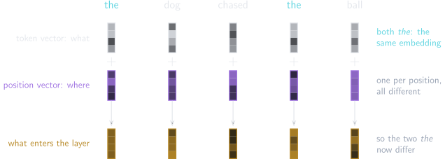
The token vector says which token is present. The position vector says where it sits.

Relative position

• Absolute: a vector per position, identifying positions 1, 2, 3, …
• Relative: information about offsets, such as “two tokens earlier”, entering the scores
  • one scheme: a learned number \(b_{m-n}\) per offset, added to \(s_{mn}\)
• For many language relationships the useful quantity is distance and direction
  • “the previous token”
  • “three tokens earlier”
  • “the matching delimiter 20 tokens back”
• Absolute positions imply these relations; relative position represents them directly
• Depending on the scheme, position changes the token representations, the compatibility scores, or both

Stabilising attention scores

Large scores and softmax

• A query–key score sums \(D_q\) terms

\[ \inner{\vect{k}}{\vect{q}} =\sum_{j=1}^{D_q}k_jq_j \]

• More terms, larger typical magnitude
• Large gaps between scores push softmax towards weights of 0 and 1
• A softmax pushed that far is saturated: near-zero gradients for most entries, so training slows
  • a weight near 0 or 1 barely moves when its score changes
• \(D_q\) is a design choice; without a correction, how sharp the softmax starts out would depend on it

Saturation

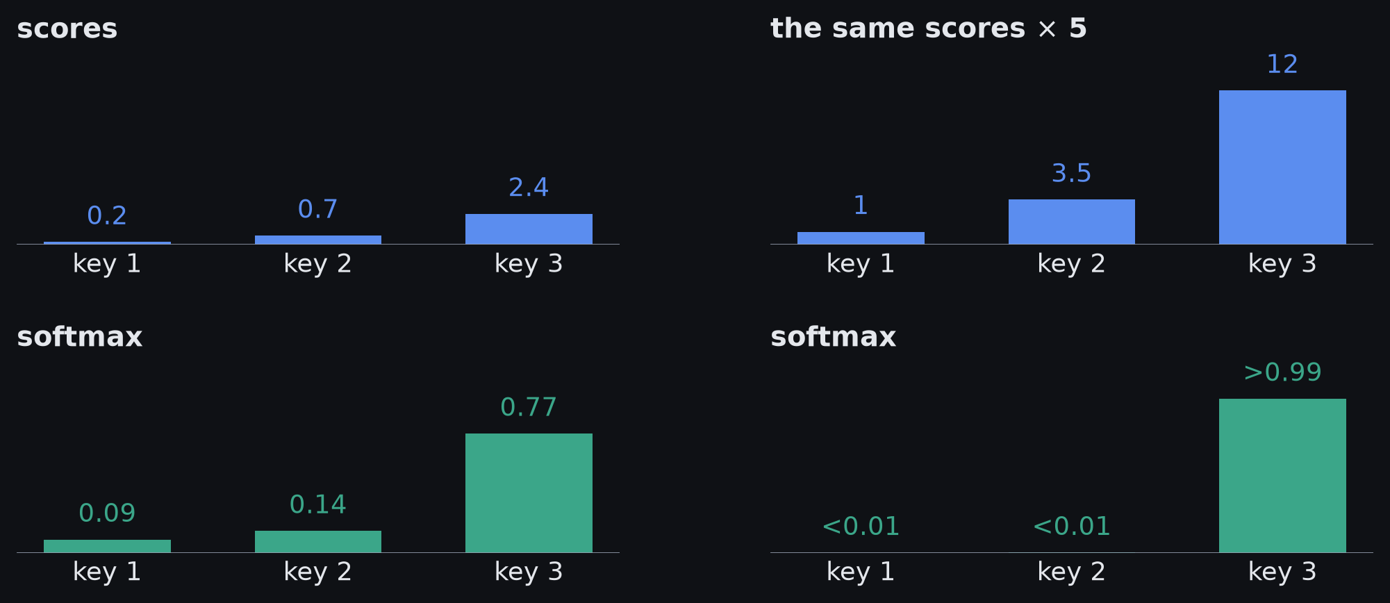
The same scores multiplied by five. Softmax now puts almost all the weight on the largest.

Score variance and dimension

• Assumption: all \(2D_q\) entries of \(\vect{k}\) and \(\vect{q}\) are independent of one another, each with mean zero and variance one
  • a model of the scores at initialisation, not a claim about a trained model
• Mean of one term: independence lets the expectation factor, so \(\expect{k_jq_j}=\expect{k_j}\expect{q_j}=0\)
• Variance of one term: with mean zero, \(\var{k_jq_j}=\expect{k_j^2q_j^2}\)
  • which factors again: \(\expect{k_j^2}\expect{q_j^2}\)
  • and with mean zero, \(\expect{k_j^2}\) is the variance of \(k_j\), so the product is \(1\times 1=1\)
• The score adds \(D_q\) such terms; the variances of independent terms add, as on Monday

\[ \var{\inner{\vect{k}}{\vect{q}}} =\sum_{j=1}^{D_q}\var{k_jq_j} =D_q \tag{14}\]

Typical score size

• Equation 14: the score’s variance is \(D_q\)
• Typical size: the standard deviation, \(\sqrt{D_q}\)
• TRY: \(D_q\) goes from 16 to 64. By what factor does the typical score grow?
• By 2, the square root of the factor of 4
• The saturation figure’s factor of 5 is what a 25-fold larger \(D_q\) would give

PROMPT: the commonest answer to the TRY is 4. Ask whether the variance or the standard deviation is the size of a typical score.

This is the square-root argument promised in week 3. Monday’s variance of a sum is the only tool it needs.

Scaled dot-product attention

Definition 6 Scaled dot-product attention divides every score by \(\sqrt{D_q}\) before the softmax.

\[ \operatorname{SA}(\mat{X}) = \mat{V} \operatorname{Softmax}_{\text{columns}} \!\left( \frac{\mat{K}\transpose\mat{Q}}{\sqrt{D_q}} \right) \tag{15}\]

• Read: “V times the column-wise softmax of K transpose Q over root D q”
• Why this divisor: dividing a variable by \(c\) divides its variance by \(c^2\), so dividing by \(\sqrt{D_q}\) returns the score’s variance to one
• What it changes: the typical score, held near one whatever \(D_q\) is, under the same assumption
• What it doesn’t: this is a stabilising scale, not extra modelling power
• In the paper: \(\softmax\!\left(\mat{Q}\mat{K}\transpose/\sqrt{\dk}\right)\mat{V}\), with tokens in rows; its \(\dk\) is Prince’s \(D_q\), and ours (Vaswani et al. 2017)

PROMPT: Monday’s reading questions on the paper. Take the main claim and the evidence for it from two or three people here, where the paper’s formula is on screen.

Multiple attention heads

One pattern per mechanism

• One self-attention mechanism gives each query one distribution over the source positions
• Attention pattern: all \(N\) of those distributions for one input, the matrix \(\mat{A}\)
• In the example, cooks needs two things: its subject, it, and its object, food
• One mechanism returns one average: with half the weight on each, \(0.5\,\vect{v}_{\text{it}}+0.5\,\vect{v}_{\text{food}}\)
  • the blend no longer says which was the subject and which the object
• Several mechanisms can retrieve the two separately, each through its own value projection
• Status: a motivating intuition; several mechanisms in parallel work better in practice, but why is not settled

Three routing patterns

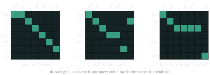
Three hand-built patterns over one sequence, not measured from a model. One self-attention mechanism gives each query a single distribution, so it cannot be all three.

Multi-head self-attention

Definition 7 Multi-head self-attention runs \(H\) self-attention mechanisms, the heads, in parallel on the same input, each with its own query, key and value projections, and then combines their outputs.

• Head \(h\) has its own projections

\[ \mat{Q}_h=\layerweights_{qh}\mat{X},\qquad \mat{K}_h=\layerweights_{kh}\mat{X},\qquad \mat{V}_h=\layerweights_{vh}\mat{X} \]

• And so its own scores and weights

\[ \operatorname{SA}_h(\mat{X}) = \mat{V}_h \operatorname{Softmax}_{\text{columns}} \!\left( \frac{\mat{K}_h\transpose\mat{Q}_h}{\sqrt{D_q}} \right) \tag{16}\]

Projections per head

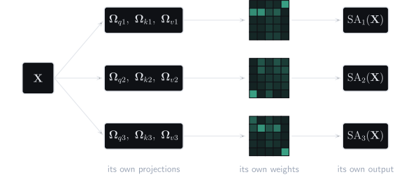
Each head has its own query, key, and value projections, and so its own weights. The three grids are random projections of one input, not trained heads.

Combining the heads

1. Compute the \(H\) head outputs in parallel
2. Concatenate them, stacking their feature dimensions
3. Mix them with a learned linear map \(\layerweights_c\), so every head can write to every entry of the output

\[ \operatorname{MHSA}(\mat{X}) = \layerweights_c \operatorname{Concat} \left( \operatorname{SA}_1(\mat{X}),\ldots,\operatorname{SA}_H(\mat{X}) \right) \tag{17}\]

• Shapes: each \(\operatorname{SA}_h(\mat{X})\) is \(D_v\times N\); the concatenation is \(HD_v\times N\); \(\layerweights_c\) is \(D\times HD_v\)
• Output: \(D\times N\), the shape of the input, whatever \(D_v\) is
• Usual choice: \(D_q=D_v=D/H\), so the concatenation is already \(D\times N\)
  • \(H\) heads of width \(D/H\) have as many projection parameters as one head of width \(D\): heads split a budget
• TRY: \(H=8\) and \(D=512\). What is \(D_q\), and what shape is the concatenation?
• \(D_q=64\), and \(512\times N\)
• In Prince: \(\mathrm{MhSa}[\mat{X}]\)

A transformer layer

From one operation to a layer

• So far: one operation, multi-head self-attention
• A transformer is a deep network made by stacking one kind of layer many times
• Attention alone is not that layer; three things are missing
  • it only moves and blends features: add an MLP at each position
  • a deep stack needs a direct route for gradients: add residual paths
  • repeated additions change the scale: add LayerNorm
• The next slides add them one at a time, then assemble the layer

What attention can’t do

• Given its weights, attention’s output is an average of linearly projected values
• It moves features between positions and blends them; it computes no new feature from them
  • after attention the vector at it holds “pronoun” and “a place that serves food” side by side, in the earlier gloss
• Making a new feature out of what has arrived takes a nonlinear function of that one vector
• MLP: week 1’s network with a hidden layer and an activation does that

The position-wise MLP

• Position-wise MLP: one small MLP, applied to each position’s vector separately
  • \(D\) entries in, a wider hidden layer with an activation such as ReLU, \(D\) entries out
• Position-wise: the output at position \(n\) depends on \(\vect{x}_n\) alone; nothing crosses between positions here
• Shared: the same parameters at every position, so any sequence length still works
• The layer’s two kinds of computation
  • self-attention, across positions: which others should contribute?
  • the MLP, within a position: how should what has arrived be combined?

Residual paths

• Until now, attention’s output replaced the vector at each position
• In a transformer it is added to that vector

\[ \mat{X} \leftarrow \mat{X}+\operatorname{MHSA}(\mat{X}) \]

• Read: “X becomes X plus the attention output”; the arrow overwrites \(\mat{X}\), as in a gradient step
• Column \(n\): what position \(n\) held, plus what attention gathered for it
• In the example: the vector at it keeps “pronoun” and gains what it drew from restaurant
  • the identity path keeps a position’s own vector, so attention’s weights are free to go elsewhere
• Monday’s block: \(\hidden_k=\hidden_{k-1}+\vect{f}_k[\hidden_{k-1}]\), with attention as the branch \(\vect{f}_k\)

• The same for the position-wise MLP

\[ \vect{x}_n \leftarrow \vect{x}_n+\operatorname{MLP}(\vect{x}_n) \]

• TRY: from Monday, what does the identity path give a deep network?
• A direct route for information and for gradients; each branch learns a change to the current representation
• Shape: adding needs matching shapes, which is why multi-head attention returns \(D\times N\)
• Residual stream: the main path through all the layers; each sublayer, attention or MLP, reads from it and adds to it

Layer normalisation

Definition 8 LayerNorm standardises one token’s vector using the mean and variance of that vector’s own \(D\) entries, then applies a learned scale and offset.

• For one token vector \(\vect{x}\) with entries \(x_1,\ldots,x_D\)

\[ m_{\vect{x}}=\frac{1}{D}\sum_{d=1}^{D}x_d, \qquad s_{\vect{x}}^2=\frac{1}{D}\sum_{d=1}^{D}(x_d-m_{\vect{x}})^2, \qquad \tilde{x}_d=\gamma_d\,\frac{x_d-m_{\vect{x}}}{\sqrt{s_{\vect{x}}^2+\epsilon}}+\delta_d \tag{18}\]

• Read: “the mean and variance of this one vector’s entries”; \(m_{\vect{x}}\) is not the source index \(m\)
• Why here: each residual addition adds variance, as on Monday; normalising after each sublayer resets the scale

• Monday’s four BatchNorm steps, with the statistics taken along a different axis

	Mean and variance over	Needs a batch
BatchNorm	one feature, across the minibatch	yes
LayerNorm	one token, across its \(D\) features	no

• Learned: one scale \(\gamma_d\) and one offset \(\delta_d\) per feature, shared by every position
• Why not BatchNorm: sequences in a batch differ in length, and generation runs one token at a time; one token’s own statistics don’t depend on the rest of the batch

The transformer layer

Definition 9 A transformer layer applies multi-head self-attention and then a position-wise MLP, each inside a residual connection and each followed by LayerNorm.

\[ \begin{aligned} \mat{X} &\leftarrow \mat{X}+\operatorname{MHSA}(\mat{X})\\ \mat{X} &\leftarrow \operatorname{LayerNorm}(\mat{X})\\ \vect{x}_n &\leftarrow \vect{x}_n+\operatorname{MLP}(\vect{x}_n)\quad \forall n\\ \mat{X} &\leftarrow \operatorname{LayerNorm}(\mat{X}) \end{aligned} \tag{19}\]

• LayerNorm of a matrix: Equation 18 applied to each column, one token at a time
• TRY: which of the four lines can move information from one position to another?
• Only the first: the MLP and LayerNorm act on one column at a time
• Post-norm: the order here, with LayerNorm after each sublayer; pre-norm, with it before, is also common
• A transformer stacks many such layers
  • a later layer’s queries can use what an earlier layer gathered: it can ask for something that cooks once cooks has reached it

One layer, drawn

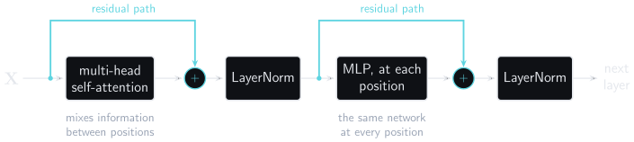
Multi-head attention moves information between positions. The MLP then transforms each position on its own. Each sublayer has a residual path and LayerNorm.

From text to embeddings

From text to vectors

• A language pipeline turns text into vectors in three steps

\[ \text{text}\rightarrow\text{tokens}\rightarrow\text{token IDs}\rightarrow\text{embeddings} \]

• Tokens: pieces of the text, cut by a tokenizer
• Token IDs: each piece’s integer index in the vocabulary, the fixed list of every piece the tokenizer can emit
• Embeddings: one learned vector per ID
• The transformer receives the embedding sequence, never characters or strings

Whole-word vocabularies

• One token per whole word has problems
  • names and rare words may be unseen
  • punctuation carries information
  • related forms such as walk, walked, walking become unrelated IDs
  • the vocabulary can become extremely large
• One token per character has no unknown words, but makes long sequences
• Subword tokenisation is a compromise between vocabulary size and sequence length.

Subword tokenisation

• A subword vocabulary mixes
  • characters or bytes
  • common word fragments
  • common complete words
• Byte-pair-style methods build it by repeatedly merging units that often sit side by side
• A rare word is spelt from pieces that appear elsewhere: un + believ + able
• Tokenizer-dependent: real boundaries depend on the tokenizer and its vocabulary; words don’t map one-to-one to tokens

Vocabulary size against sequence length

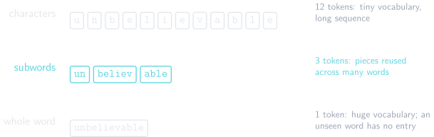
Frequent fragments become single tokens, and rare words are built from smaller pieces. Whole words would need a huge vocabulary; characters would give long sequences.

Embedding lookup

Definition 10 An embedding is the learned vector a model stores for one vocabulary item. The embedding matrix \(\layerweights_e\in\reals^{D\times|\set{V}|}\) holds one per column, for a vocabulary \(\set{V}\).

• A one-hot vector \(\vect{t}_n\in\reals^{|\set{V}|}\) marks which token sits at position \(n\)

\[ \vect{x}_n=\layerweights_e\vect{t}_n \tag{20}\]

• Read: “Omega e times a one-hot vector”: the product picks out one column
• Shape: \((D\times|\set{V}|)(|\set{V}|\times 1)\rightarrow D\times 1\)
• In software: an index into the matrix, called an embedding lookup; no dense product is formed

Lookup as column selection

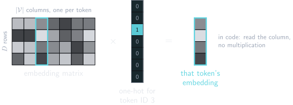
Lookup equals multiplying the embedding matrix by a one-hot vector. Implementations select the column directly.

Repeated tokens

• The same token gets the same learned vector wherever it occurs: bank in river bank and in loan from the bank
• After positional information and transformer layers
  • the two positions differ
  • each attends to different context

Definition 11 A contextual embedding is the representation at one position after transformer layers have mixed in information from the rest of the sequence.

One token, different contextual embeddings

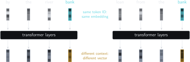
The same token ID starts from the same embedding. Different context to its left makes its contextual embeddings differ.

Encoder models

Encoders

• An encoder uses self-attention exactly as defined so far
  • every token can attend to every other token
  • each output representation can use left and right context
• The result is one contextual embedding per position, each drawing on the complete input
• Useful when the whole input is available before the task output is produced
  • text classification
  • named-entity recognition
  • extractive question answering

Bidirectional context

The [MASK] pulled into the station.

• TRY: what fills the mask, and which words told you?
• Left context: The …
• Right context: … pulled into the station
• train, most likely: the right context did the work; an encoder can use both sides
• Restoring a hidden token rewards representations that carry what is needed to restore it

Masked-token prediction

1. Take an ordinary text sequence
2. Replace a subset of its tokens with a special mask token
3. Run the encoder
4. Predict the original token at each masked position, with a linear layer and softmax over the vocabulary, as in week 2’s classifier

• No human annotation is needed: the text supplies its own targets
• Self-supervised learning, as in week 4: supervision constructed from the data itself
• This is the pre-training task of BERT-like models
• Scope: good masked-token prediction shows learned statistical structure; it doesn’t by itself establish human-like understanding

Masked-token pre-training

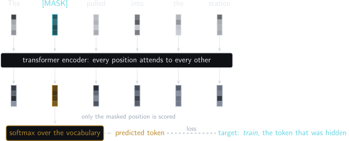
The encoder sees context on both sides of the masked position and is trained to recover the hidden token. The text needs no labels.

Fine-tuning

• After pre-training, attach a small task-specific output layer and train on labelled examples
  • text classification: map the output at the class token, a special token placed first in every input, to class logits
    • its position can attend to every other, so training can make it a summary
  • named-entity recognition: map each token’s output to entity-type logits
  • extractive question answering: predict the start and end positions of the answer span
• TRY: from week 4’s transfer learning, which parameters start from pre-training and which start fresh?
• The encoder starts pretrained; the new output layer starts fresh
• Pre-training learns reusable features; fine-tuning adapts them to a narrower task

A concrete encoder: BERT

• The BERT configuration Prince describes (Prince 2023)
  • a 30,000-token vocabulary
  • 1024-dimensional token representations
  • 24 transformer layers
  • 16 attention heads per layer
  • 64-dimensional queries, keys, and values per head
  • an MLP hidden dimension of 4096
  • about 340 million parameters
• The usual choice at work: 16 heads of 64 entries concatenate back to 1024
• MLP: its hidden layer is four times the model width
• One historical design point, not part of the definition of an encoder

Decoder models and language modelling

Next-token prediction

• TRY: It takes great … what comes next, and how sure are you?

Definition 12 An autoregressive language model returns, for any prefix \(t_1,\ldots,t_n\), a probability distribution over the next token \(t_{n+1}\).

\[ \prob{t_{n+1}\mid t_1,\ldots,t_n} \tag{21}\]

• Read: “the probability of token n plus one, given the n tokens before it”
• \(t_n\): the token at position \(n\); its one-hot vector is \(\vect{t}_n\)
• A decoder is a transformer that computes it: built like the encoder, with one restriction on attention, below
• Repeating the prediction, one token at a time, generates a sequence

Logits and the next-token distribution

• At position \(n\), the last layer outputs a contextual embedding \(\vect{x}_n\)
• A learned output layer gives one logit per vocabulary item

\[ \vect{z}_n = \layerbias_{\text{out}}+\layerweights_{\text{out}}\vect{x}_n, \qquad \vect{z}_n\in\reals^{|\set{V}|} \tag{22}\]

• Softmax turns the logits into the next-token distribution

\[ \prob{t_{n+1}\mid t_1,\ldots,t_n} = \softmax(\vect{z}_n) \tag{23}\]

• Shape: \(\layerweights_{\text{out}}\) is \(|\set{V}|\times D\)
• Offset: position \(n\) predicts token \(n+1\), so \(\vect{x}_n\) must depend on tokens \(1,\ldots,n\) only; causal masking, below, enforces that

From contextual embedding to probabilities

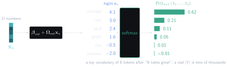
The contextual embedding is projected to one logit per vocabulary item. Softmax turns the logits into the next-token distribution.

The chain rule of probability

• Two events first: \(\prob{a,b}=\prob{a}\prob{b\mid a}\)
• The chain rule of probability repeats that step: any joint distribution is a product of conditionals

\[ \prob{t_1,\ldots,t_N} = \prob{t_1} \prod_{n=2}^{N} \prob{t_n\mid t_1,\ldots,t_{n-1}} \tag{24}\]

• Read: “the product, for n from 2 to N, of each token’s probability given the ones before it”
• TRY: write out the factors for It takes great
• \(\prob{\text{It}}\,\prob{\text{takes}\mid\text{It}}\,\prob{\text{great}\mid\text{It takes}}\)
• Not the calculus chain rule: no derivatives here
• An identity: true of every distribution over sequences
• An autoregressive language model estimates every factor with the same network

One sentence, many examples

It takes great courage …

• Every prefix is a training example, with the next token as its target
  • It → takes
  • It takes → great
  • It takes great → courage
• One pass per prefix: correct, but it recomputes the shared prefix every time
• The goal: one pass over the whole sentence, in which the output at position \(n\) is what the pass over its prefix alone would have given

Leakage in parallel training

It takes great courage …

• The prediction of great is read off the position of takes, the token before it
• With unrestricted self-attention over the whole sentence, that position can attend to
  • great itself, one position later
  • every token after it
• The model would use information it won’t have when generating
• We need parallel training over the whole sequence, with no information flowing back from the future.

Causal masking

Definition 13 A causal mask sets the score \(s_{mn}\) to \(-\infty\) whenever the source position \(m\) is later than the destination position \(n\), before the softmax.

\[ s_{mn}=-\infty \quad\text{when }m>n \tag{25}\]

• \(\exp(-\infty)=0\), so those attention weights are exactly zero
• The remaining weights for query \(n\) still sum to one: the softmax runs over what is left
• Position \(n\) may use positions \(1,\ldots,n\), itself included
• All positions are still processed in parallel during training
• In Prince: masked self-attention; not the mask token of encoder pre-training

The causal triangle

• The convention of \(\mat{K}\transpose\mat{Q}\): rows are keys, at source positions \(m\); columns are queries, at destination positions \(n\)
• TRY: four tokens. Mark each cell of the \(4\times 4\) grid as kept or masked
• Query \(n\) keeps the keys with \(m\le n\)

\[ \begin{bmatrix} \checkmark & \checkmark & \checkmark & \checkmark\\ \times & \checkmark & \checkmark & \checkmark\\ \times & \times & \checkmark & \checkmark\\ \times & \times & \times & \checkmark \end{bmatrix} \]

• Convention: libraries that store tokens in rows show the transpose of this triangle
  • remember the rule, not the picture: query \(n\) cannot use keys from positions later than \(n\)

PROMPT: students draw the grid before the reveal. A lower triangle is the row-token convention, and is the right answer to a different layout; ask which axis they put the queries on.

Causal masking on the grid

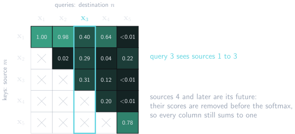
The same sequence under a causal mask. Rows are keys and columns are queries. Each query keeps only its current and earlier keys.

The next-token loss

• At each position the decoder produces logits and a softmax distribution over the vocabulary
• TRY: from week 2, what does the cross-entropy loss charge when the correct class has probability \(p\)?
• \(-\log p\): the negative log-likelihood of the correct token
• Training minimises the sum, or mean, over positions

\[ \loss = -\sum_{n} \log \prob{t_{n+1}\mid t_1,\ldots,t_n} \tag{26}\]

• Every position with a next token contributes a term
• Where it comes from: take \(-\log\) of Equation 24
  • the log of a product is the sum of the logs, so each factor becomes one term
  • the sum above indexes the same terms by the length of the prefix
  • the first factor, \(\prob{t_1}\), has no prefix; in practice a fixed start-of-sequence token is placed first, so \(t_1\) is predicted too

Training and generation

• Training: every position at once
  • the ground-truth prefix is available
  • causal masking prevents look-ahead
  • many next-token losses are computed in parallel
• Generation: one token at a time
  • begin with a prompt
  • predict a distribution for the next token
  • choose or sample one token
  • append it and repeat
• Generation is sequential because each prediction depends on the tokens generated so far

Parallel training, sequential generation

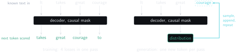
Under a causal mask, one training pass scores the next token at every position. Generation must choose a token before it can form the next distribution.

Decoding

• Given next-token probabilities, a selection rule is still needed; take the earlier distribution after It takes great
  • greedy decoding: choose the most probable token; always courage here
  • sampling: draw according to the distribution; courage 62% of the time, and now and then banana
  • top-\(k\) sampling: sample only among the \(k\) highest-probability tokens; with \(k=3\), never banana
  • beam search: keep several candidate sequences, looking for a high joint probability, which greedy choices don’t guarantee
• The network defines conditional probabilities; the decoding algorithm turns them into an output sequence.

A concrete decoder: GPT-3

• The GPT-3 configuration Prince describes (Prince 2023)
  • context length: 2048 tokens
  • 96 transformer layers
  • embedding dimension: 12,288
  • 96 attention heads
  • query, key and value dimension: 128 per head
  • 175 billion parameters
  • trained on 300 billion tokens
• The same decoder ingredients: embeddings, positional information, causal attention, MLPs, residual paths, and next-token prediction

In-context learning

• Large decoder models can sometimes perform a task from examples placed in the prompt, with no parameter update
• Few-shot, or in-context, learning is the usual name
• Performance can be erratic
• A successful continuation doesn’t reveal whether the model
  • inferred a general rule
  • interpolated from training patterns
  • reproduced memorised material
• Status: an observed capability; not evidence that gradient-based learning happens inside the model at inference time

Encoder–decoder models

Two contexts for translation

• For machine translation
  • the encoder reads the complete source sentence
  • the decoder generates the target sentence left to right
• A target token should depend on
  • the earlier target tokens
  • the encoded source sentence
• The encoder–decoder design supplies these with causal self-attention, plus a second attention mechanism over the encoder’s outputs
  • each decoder layer runs causal self-attention, then that second mechanism over the encoder’s final outputs, then the MLP

Cross-attention

Definition 14 Cross-attention computes attention with the queries taken from one sequence and the keys and values taken from another.

• Self-attention: queries, keys and values all come from the same sequence
• Encoder–decoder cross-attention
  • decoder queries ask what source information is needed now
  • encoder keys decide which source positions match
  • encoder values supply the retrieved source information
• TRY: 5 target tokens so far and 7 source tokens. What shape is the score matrix?
• \(7\times 5\): one row per encoder key, one column per decoder query, and each column’s weights sum to one over the source

Cross-attention: queries, keys and values

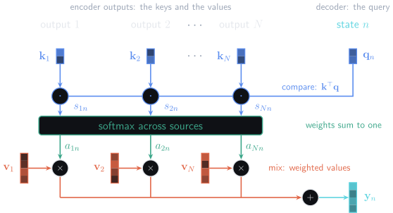
Decoder states supply the queries. Encoder states supply the keys and the values.

Three architectures

Architecture	Attention access	Typical objective or use
Encoder	whole input	build representations
Decoder	current and earlier tokens only	autoregressive generation
Encoder–decoder	source fully visible; target causal	sequence-to-sequence generation

• The same attention machinery, reused with different connectivity constraints and training objectives

Cost and long sequences

Quadratic cost

• With \(N\) tokens, the score matrix has \(N\times N=N^2\) entries
• TRY: the sequence doubles in length. What happens to the number of scores?
• \((2N)^2=4N^2\): four times as many
• Computation and memory both pay, which is the practical limit on long contexts

Doubling the sequence length

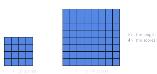
Full attention has one score per query–key pair. Going from N = 4 to N = 8 takes the grid from 16 cells to 64.

Causal masking and cost

• A decoder attends only to current and earlier tokens, which keeps just over half of the \(N^2\) interactions

\[ \frac{N(N+1)}{2}=\mathcal{O}(N^2) \]

• Read: “of order N squared”: for large \(N\), at most a fixed multiple of \(N^2\)
• Masking changes the constant factor; growth is still quadratic

Sparse attention

• One family of approaches keeps only selected interactions
  • local neighbourhoods
  • dilated patterns
  • blockwise attention
  • a small number of global tokens
  • mixtures of local and global connectivity
• Fewer pairwise comparisons, but information may need several layers to travel between distant positions
• TRY: where did week 4 meet local operations that become long-range by stacking?
• Convolutional receptive fields

Sparse attention patterns

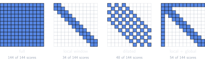
Local, dilated, and global-token patterns each keep fewer direct interactions, so each costs less to compute.

Transformers beyond text

ImageGPT

• The decoder idea extends directly: flatten an image into a pixel sequence and predict the next pixel token
• ImageGPT, as Prince describes it (Prince 2023)
  • predicts pixels autoregressively in raster order
  • quantises colour to 512 possible values, the finite vocabulary a softmax needs
  • is limited to small images by quadratic attention cost, with one token per pixel
  • can also use its learned internal representations for classification
• It works, but discards much of the 2D structure that a convolutional network is given as an architectural prior

Pixels as tokens

• An image can be treated as a sequence, but one token per pixel makes \(N\) very large
• A \(224\times224\) image has \(N=50{,}176\) pixels, before colour channels
• Full pixel-level self-attention is far too expensive
• Vision transformers need a more economical unit than one token per pixel.

ViT: patches as tokens

• The Vision Transformer, ViT, cuts an image into non-overlapping patches, for example \(16\times16\) pixels
• Each patch is
  1. flattened
  2. linearly projected to an embedding
  3. given positional information
  4. processed by a transformer encoder
• A \(224\times224\) image then has \(N=14\times14=196\) patch tokens, not 50,176 pixel positions
• The encoder also receives a class token, as BERT does; its output is classified

ViT: from image to token sequence

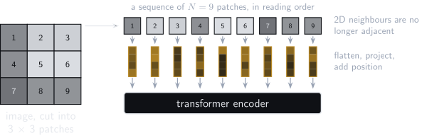
A toy image of three patches by three. The image is cut into fixed-size patches. Each patch is flattened and projected to an embedding, position is added, and the sequence enters a transformer encoder. The class token is not drawn.

Inductive bias

• A convolutional network builds in assumptions
  • local connectivity
  • shared filters
  • translation equivariance
• A basic ViT imposes less spatial structure
  • it can model global interactions early
  • it often benefits from large-scale pre-training
  • locality and multi-scale structure must be learned, or reintroduced by the architecture
• Status: empirical; data needs and relative performance depend on architecture, training recipe, dataset scale and task

Multi-scale vision transformers

• Shifted-window transformers restrict attention to local windows, then move the windows from layer to layer
  • local attention lowers cost
  • shifted windows let information cross the previous boundaries
  • periodic downsampling builds a hierarchy of spatial scales
• This recovers some of the structure familiar from convolutional networks, and keeps attention-based interactions

Putting the mechanism together

Attention as routing

• For each destination position
  • the query represents what the destination is looking for
  • the keys represent how candidate sources can be matched
  • query–key dot products give compatibility scores
  • softmax turns the scores into contribution weights
  • the values carry the information the weights route
  • the output is a weighted mixture of values
• The same core sits behind encoder attention, causal decoder attention, and cross-attention

Across positions and within them

	Component	What it does
Across positions	multi-head attention	moves and mixes information between tokens
Within positions	shared MLP	transforms the features of each token on its own

• Residual paths and normalisation make these layers practical to stack deeply

The constraints

• Variable-length sequences
• Shared processing across positions
• Long-range, content-dependent interactions
• Efficient parallel training

The choices that meet them

• Variable-length sequences → shared projections, and one output per input position
• Shared processing across positions → the same projections and MLP everywhere
• Long-range, content-dependent interactions → self-attention, all-to-all
• Efficient parallel training → no recurrence across positions; causal masking in a decoder

What the choices then need

• Attention ignores order → positional information
• Scores grow with \(D_q\) → scaling by \(\sqrt{D_q}\)
• One pattern per mechanism → multiple heads
• Many stacked layers → residual paths and LayerNorm
• All-to-all scores → cost that grows as \(N^2\)

Revision

Query, key and value: three roles

• TRY: without looking back, what is each of the three for?
• Query: what this destination position seeks
• Key: what each source position can be matched on
• Value: what each source position contributes
• Matching a source and retrieving its payload are different jobs
• Not three copies of the embedding: three separately learned projections of the same input vector

Score and weight

• TRY: which of the two can be negative, and which sums to one?
• Score: \(s_{mn}=\inner{\vect{k}_m}{\vect{q}_n}\), any real number
• Weight: \(a_{mn}=\softmax_m(s_{mn})\), non-negative, and summing to one over the sources for each query
  • strictly positive unless masked

Self-attention, causal attention, and cross-attention

• TRY: in a translation model’s cross-attention, which of queries, keys and values come from the encoder?
• Self-attention: queries, keys and values come from the same sequence
• Causal self-attention: self-attention plus a mask that blocks future positions
• Cross-attention: queries come from one sequence; keys and values from another
  • in translation: queries from the decoder, keys and values from the encoder
• The weighted-retrieval computation is the same in all three

Tokens, embeddings, and contextual embeddings

• Token: a discrete vocabulary item
• Token ID: its integer index
• Embedding: the learned vector stored for that ID
• Contextual embedding: the vector at one position after attention has mixed in its surroundings
• The same token ID can end with different contextual embeddings in different sequences

Encoder and decoder objectives

• Encoder pre-training: restores masked content using context in both directions
• Decoder training: predicts each next token from its permitted prefix only
• Encoder–decoder: conditions target generation on the source representations and the earlier target tokens
• Two masks: the mask token replaces an input; the causal mask removes scores
• TRY: write the causal mask for \(N=3\) as a grid of kept and masked cells
• Kept on and above the diagonal: query \(n\) keeps the keys with \(m\le n\)
• Architecture and objective together fix the task; “transformer” alone doesn’t

Four equations to recognise

• Scaled attention scores: \(\mat{K}\transpose\mat{Q}/\sqrt{D_q}\)
• Attention output, Equation 15: \(\mat{V}\operatorname{Softmax}_{\text{columns}}\!\left(\mat{K}\transpose\mat{Q}/\sqrt{D_q}\right)\)
• Autoregressive factorisation, Equation 24: \(\prob{t_1,\ldots,t_N}=\prob{t_1}\prod_{n=2}^{N}\prob{t_n\mid t_1,\ldots,t_{n-1}}\)
• Next-token negative log-likelihood, Equation 26: \(\loss=-\sum_n \log \prob{t_{n+1}\mid t_1,\ldots,t_n}\)

Reading attention weights

Weights as explanations

• Attention weights are easy to plot, and a plot invites “the model looks at restaurant”
• Is a weight evidence of how the model computes its answer?
• A test needs a model small enough that we can cut one weight and measure again

A model small enough to read

• Two of today’s layers, one attention head each, trained on a lookup task
  • causal masking, as in a decoder; learned positional encodings
• Input: 4 letter–digit pairs, then one of the letters again: c 5 a 2 f 7 b 0 a
  • letters are distinct; digits may repeat
• Target: the digit that followed that letter, here 2; read from the last position’s output, as in next-token prediction
• Naming: the task looks like a dict, but letters aren’t keys and digits aren’t values here; those words stay with attention’s projections
• Result: 100% of 4,000 freshly drawn sequences correct, in each of 3 training runs

One attention step

• TRY: can one attention step solve this? What does the last position hold, and where is the answer?
• The last position holds a letter; its query can match that letter’s earlier copy
• The answer sits one place to the right of that copy, in a vector that holds a digit and no letter
  • so the scores have nothing to pick the answer out by
  • the query can’t ask for “the position after my letter’s copy” before it has found the copy
• Measured: the same model with one layer gets 42%, mean of the runs
• Three guesses: any digit, 1 in 8; a digit in the sequence, 35%; the sequence’s most frequent digit, 43%
  • one layer does no better than the third, which never uses the asked letter
• What two steps could do: first put each letter into the vector of the digit after it; then the last position’s query can match that digit directly

PROMPT: give the TRY a minute in pairs. The point to draw out is that the last position can match its letter by content, and that the answer is then somewhere else.

Two patterns from the trained model

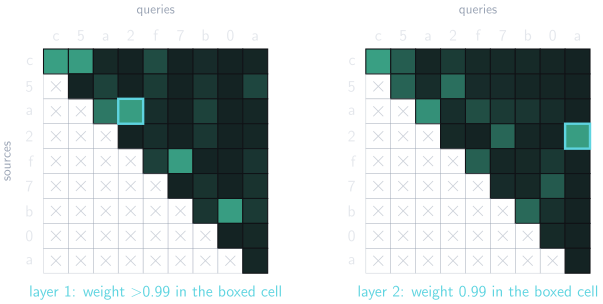
Attention weights from one of the three trained models, for one sequence, one grid per layer. Rows are sources and columns are queries. The boxed cells are the two steps of the lookup. In layer 2 only the last column feeds the output. Crossed cells are scores the causal mask removes.

Reading the two patterns

• Layer 1: each digit gives almost all its weight to the letter just before it
  • 0.99 on average, over the test sequences and the runs
• Layer 2: the last position gives 0.99 of its weight to the digit that followed its own letter, in this sequence
• Each is a pattern a person can name: “the previous token”, and “my letter’s digit”
• The story they suggest: layer 1 adds the first a to the vector at 2, by the residual sum; layer 2 computes its key at 2 from that vector, so the last a can match it
• What a column says: which sources that position drew value vectors from, in this head, for this input
• A pattern can’t say whether that story is how the model works; an experiment can

The route the patterns suggest

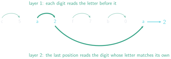
The two steps the patterns suggest. Layer 1 copies each letter into the digit after it; layer 2 lets the last position find the digit carrying its own letter.

Testing a weight: cut it

• Is the large layer-2 weight what produces the answer? Remove it and measure again

Definition 15 An intervention changes one part of a running model and measures what happens to its output.

• Here: remove one source from one query’s softmax, by setting its score to \(-\infty\)
  • the causal mask’s operation, applied on purpose; the remaining weights renormalise
• TRY: in layer 2, stop the last position reading the matching digit. Predict the accuracy; guessing any digit gets 1 in 8

PROMPT: collect three or four predicted accuracies before the next slide. “About half” is common; ask what the model has left to go on.

Layer 2, at the last position	Accuracy, mean of the runs
none	100%
cut the matching digit	14%
cut a different digit	100%

• Control: the third row; cutting a weight isn’t what hurts, cutting this one is
• Here the large weight is doing the work: without it the model is close to guessing.

Testing the other weights

• The layer-2 weight mattered; does every weight? The last position also attends in layer 1
• In layer 1 the last position spreads its weight: averaged over the test sequences and the runs, about 0.17 on each digit, the matching one included
• Cut its largest layer-1 weight, whichever source that is: accuracy 100%
• Replace all of them with a uniform distribution: 100%
• Remove layer 1’s whole attention update at the last position, the attention term of its residual sum: 100%
• So the answer doesn’t depend on what those weights bring in
  • these weights are small and spread; the next slide has the sharper case
• A weight says information was mixed in, not that the output used it.

A hidden step

• In the example, the last position’s layer-2 column points at one cell: the digit 2
• Nothing in that column shows why 2 matched
  • the patterns suggest that layer 1 had copied the a before it into its position
• In every test sequence, cut the layer-1 weight the matching digit gives its own letter: accuracy falls to 36%, mean of the runs
  • guessing a digit in the sequence gets 35%
  • the layer-2 cut did worse: it hides the answer’s digit itself, where this cut leaves all four digits in view
• In layer 2 the last position gives that earlier letter 0.1% of its weight, on average
  • the answer depends on the letter all the same, by way of the digit layer 1 copied it into
  • a weight near zero, on a token the answer can’t do without
• One head’s pattern shows one step of a computation, not the computation.

Attention weights as evidence

Claim	Does a weight alone support it?
position \(n\) drew on source \(m\) in this head	yes: that is Definition 1
source \(m\) mattered to the output	no: needs an intervention
this head carries out a nameable relation	no: needs many inputs, and interventions
the model “pays attention” as a person does	not a claim a weight addresses

• The output is weight times value, Equation 6, and then an MLP: the weight is one factor
• Reading heads: some show patterns a person can name; a head is a learned component, with no guarantee of a nameable role

Beyond this model

• Scope: one small model on one task; the method carries over to large models, the particular findings need not
• An early measurement: in recurrent text models with an attention layer added, attention weights often disagreed with other measures of importance (Jain and Wallace 2019)
• The reply: whether that disqualifies them depends on what the explanation is for (Wiegreffe and Pinter 2019)

Which claim does the weight support?

• TRY: in some large model, one head sends most of the weight at it to restaurant. Which of these follow?
  1. at it, that head gave the value from restaurant most of the weight in its mixture
  2. the model has worked out what it refers to
  3. cutting that weight would change the model’s answer
• Only the first, which restates the weight
  • the third needs an intervention; the second needs many inputs as well
• The habit: say what the evidence is evidence of, then say what would test the rest

The habit is the bridge into the coda. There the evidence is a model’s own sentences. The same two moves apply: say what it is evidence of, then what would test the rest.

Coda: language, meaning, and mind

Two questions

• The same habit, with new evidence: the evidence is now the model’s own sentences
• People will tell you “it understands me” and “it’s only autocomplete”; each goes beyond what the mechanism shows
• Question one: does a language model’s output mean anything to the model?
• Question two: does the model experience anything?
• An answer to one is not an answer to the other; neither is settled
• The route: vocabulary from linguistics, then three readings of question one, then six positions on question two
  • for each, its best case and its hardest objection
• TRY: write your own answer to each question, one line apiece. We come back to them

Collect nothing yet. The two lines are for the last slide.

Saussure’s sign

• Saussure, a linguist lecturing around 1910, split a word into two parts; the split lets us say what a model is given and what is in dispute

Definition 16 A sign joins a signifier, the sound pattern as a speaker holds it in mind, to a signified, the concept it calls up.

• Instance: the sound or spelling tree is the signifier; the concept of a tree is the signified; the oak outside is neither
  • later writers call the thing in the world the referent; both sides of the sign are in the speaker’s mind (Saussure 1959)
• Arbitrary: nothing about the form tree suits it to the concept
• Token IDs: a token ID plays the signifier’s part, a form with no built-in tie to a concept
  • renumber the vocabulary, reorder the embedding matrix and the output layer to match, and the model is unchanged
  • extending Saussure to written tokens is this course’s gloss
• Question one, restated: a model is given signifiers; does it come to have signifieds?

Value: differences without positive terms

• French mouton covers what English splits into sheep and mutton, so mouton and sheep can name the same animal and still differ in value (Saussure 1959)
• Value: a sign’s place in the system, fixed by its contrasts with the other signs
  • Saussure’s word; nothing to do with attention’s value vectors
• Saussure: “in language there are only differences without positive terms”
  • a positive term would have content of its own, apart from the system
• This course’s gloss: an embedding fits the description
  • no single coordinate means anything on its own; what the layers use is how the vector relates to other vectors
  • the training signal contains nothing but other tokens
• One side only: a model is trained on signifiers alone, closer to distributional linguistics, the later view that a word’s meaning shows in the contexts it occurs in
  • for the case that embeddings continue Saussure’s structuralism, see Gastaldi (2020)

Saussure’s own caveat, if asked: the slogan holds for each side taken separately; the two-sided sign as a whole he calls “positive”.

Two kinds of relation, two softmaxes

• In the example sentence, restaurant stands beside refused; it stands in place of café or hotel, which could have been there

Saussure’s relation	Holds between	In a transformer
syntagmatic	signs present together in the chain, the sequence	attention weights: a distribution over positions
associative	a sign and the absent signs it calls to mind	the next-token distribution: a distribution over the vocabulary

• What it buys: the two softmaxes answer different questions, which present token to draw on and which absent token belongs here
• Next-token and masked-token prediction both train the second: fill the slot
• Status: the two relations are Saussure’s (Saussure 1959); the mapping is this course’s gloss, not his claim

If asked: later structuralists narrow the associative kind to the signs that could fill the same slot, and call it paradigmatic.

Lacan: meaning after the fact

• TRY: The bank … What does bank mean? Now add … was steep and muddy
• Lacan, a psychoanalyst reworking Saussure, has a name for what happened: until a sentence ends, the sense of its words slides; its last term fixes them, at a point de capiton, a “button tie” in Fink’s translation (Lacan 2006)
• What is new here: direction in time; later tokens settle earlier ones, and the two architectures do it differently
• In an encoder: the later words change the representation at bank itself
• In a decoder: the vector at bank is fixed once computed; later positions settle its sense by how their queries read it
• Status: our gloss on the mechanism; Lacan’s theory concerns speaking subjects, and none of that carries over

PROMPT: take “river” and “money” answers to the first half before showing the continuation. Then ask which architecture from earlier today could revise its first reading.

Reading one: relational meaning

• The first of three answers to question one
• Claim: meaning is an internal state’s role among other states, so a model that gets the roles right has much of it (Piantadosi and Hill 2022)
  • the vector for restaurant means what it does through its relations to those for serve, menu and cooks
• Best case: structure nobody labelled turns up in models trained on token sequences alone
  • colour words arranged in a way that significantly matches human colour perception (Abdou et al. 2021)
  • a model shown only Othello moves holds a representation of the board (Li et al. 2022)
• Hardest objection: a dictionary defines words only with words; learn Chinese from a Chinese–Chinese dictionary and you never reach the world (Harnad 1990)
  • this is the symbol grounding problem: how symbols connect to what they are about, and not only to other symbols
• The slogan it challenges: “it’s only autocomplete”

The Chinese Room

• Searle’s thought experiment (Searle 1980)
  • a person who knows no Chinese sits in a room with a rule book
  • Chinese questions come in; the person follows the rules and passes Chinese answers out
  • from outside the answers are fluent; inside, nobody understands a word
• The mapping: the rule book is the program; the person is the processor
• Searle’s claim: running a program is not enough for understanding
• The standard reply: perhaps the whole room understands, though the person in it doesn’t

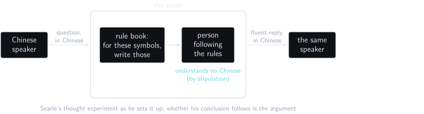
Following rules, the person turns Chinese input into convincing Chinese output and, by stipulation, understands none of it.

Reading two: form without meaning

• Claim: meaning relates a form to something outside language, the speaker’s communicative intent, and training on form alone can’t supply that relation (Bender and Koller 2020)
• Best case: next-token prediction rewards fit to text; nothing in the objective rewards truth or reference
  • their octopus taps a cable between two islanders and learns to predict their replies; it can’t help when one of them meets a bear
  • the Chinese Room reaches the same conclusion by another route
• Hardest objection: if meaning is defined as a tie to something outside language, the conclusion follows from the definition, so the argument is only as good as that definition
  • the reading still owes an account of why form alone gets so much right
• The slogan it challenges: “it obviously understands me”

Reading three: inherited grounding

• Claim: text is written by people in contact with the world, so a model’s internal states can be about the world at second hand (Mollo and Millière 2023)
  • as you can hold true beliefs about a city you have never visited, from what visitors wrote
• Best case: those states carry information about the world, and training kept them because they do: states that track the world predict text better
• Hardest objection: the model can check a sentence against nothing but more text; contact at second hand may not be contact
• The slogan it challenges: “it has never seen a tree, so tree means nothing to it”

Three readings, side by side

Reading	Does the output mean anything to the model?
relational	yes: meaning is in the relations
form without meaning	no: form is all it has
inherited grounding	yes, at second hand

• All three have serious defenders
• Question two is separate from all of them

Meaning and experience

• There is something it is like to taste coffee or to have a toothache; a camera registers red with, presumably, nothing it is like to see it

Definition 17 A system is phenomenally conscious if there is something it is like to be that system: experience from its own point of view.

• Source: the phrase is Nagel’s, from asking what it is like to be a bat (Nagel 1974)
• Subject: whatever has such experience
• Grant the most generous reading: the model’s states mean something; nothing follows yet about experience
• Often run together with experience: intelligence, a model of itself, goals, fluent first-person language
  • a chess engine is capable, but nobody presumes it feels anything
  • contested: some theories make a self-model or agency part of what consciousness is (Butlin et al. 2023)
• Encoding signs and their meanings is one claim; having experience is another.

How do you know that I am conscious?

• TRY: you can’t observe my experience. What convinces you it is there?
• I am biologically and behaviourally like you
• I report pain, memory, intention, fatigue and pleasure
• Those reports sit inside long interaction with a shared world
• My behaviour changes coherently with injury, perception and circumstance
• You know from your own case that a creature built like this can be conscious
• Strong evidence, but still an inference: the problem of other minds.

PROMPT: ask the room for reasons before revealing the bullets.

The same sentence, five producers

I don’t want to die. Please don’t kill me.

1. Printed on a sheet of paper
2. Played from a fixed recording
3. Emitted by a simple scripted program
4. Generated responsively by a language model
5. Spoken to you by another person

• TRY: where does your confidence in a frightened subject change, and what evidence changed it?
• The sentence is the same in all five; what differs is everything else you know about what produced it

PROMPT: ask for a show of hands at each of the five. Then ask someone who changed between two of them to name the evidence that moved them.

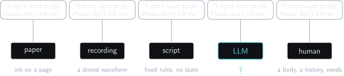
The same first-person sentence can come from systems with very different causal organisation. The sentence alone doesn’t say which of them has the experience.

Self-report

• One mechanism: a decoder produces Paris is the capital of France and I don’t want to die the same way, Equation 23
• Why that matters: the model was trained to continue human text, which is full of first-person reports; it would write the sentence whether or not anything is felt
  • evidence that turns up either way can’t tell the two cases apart
  • a system trained to mimic people can pass behavioural tests while working quite differently (Butlin et al. 2023)
• What the second sentence shows: linguistic capability; it has the form of fear
• What it doesn’t show: that fear lies behind it
• Nor the reverse: explaining how a sentence was generated doesn’t show that no experience is there
• The habit again: say what the sentence is evidence of, then what would test the rest

Six positions on machine consciousness

• Question two: does the model experience anything?
• Each position says what consciousness is, and so what would settle the question for a machine
• One slide each: what it says, its verdict on machines, its best case, its hardest objection
• For each, ask whether what settles it is something a transcript could show
• Status: each case and objection is a standard argument compressed to a line, unless marked as this course’s own

Computational functionalism

• What it says: consciousness is a kind of computation, so whatever runs the right computation has it (Butlin et al. 2023)
• For a machine: possible
  • a working assumption, not a yes; one expert review finds no current system a strong candidate, but no obvious technical barrier
• Best case: what a part of the brain contributes is what it does, so the same doing in another material should serve
• Hardest objection: a simulated storm leaves nothing wet (Searle 1980); why would simulated processing be experience?

Biological naturalism

• What it says: consciousness is caused by the brain’s physical processes, as photosynthesis is by a leaf’s; a program only describes such processes (Searle 1980)
• For a machine: not by running a program; a machine with the right causal powers would qualify
  • the 1980 paper argues about understanding; this deck applies it to experience
• Best case: every system known to be conscious is a living brain
• Hardest objection: which causal powers? Nothing yet picks them out, so nothing says which artefacts would have them

Integrated information theory

• What it says: consciousness is integrated information, how far a physical system’s parts constrain one another as a single whole beyond what they do separately (Tononi and Koch 2014)
• For a machine: the hardware’s causal structure decides, not the software
  • a little experience for very simple systems; almost none for a conventional computer, whatever it simulates
• Best case: it starts from experience and derives what a physical system must be like to have it, so it doesn’t assume that brains are special
• Hardest objection: its starting axioms are disputed, and the quantity it rests on can’t be computed for a real system

Panpsychism

• What it says: experience is a basic feature of matter, present in some small measure everywhere (Goff et al. 2022)
• For a machine: the chips’ atoms have some; that doesn’t make the model a subject
• Best case: it needn’t explain how experience arises from matter that has none
• Hardest objection: how small experiences combine into one subject is unsolved

Substance dualism

• What it says: mind is a non-physical substance, distinct from the body (Robinson and Weir 2025)
• For a machine: matter alone doesn’t make a mind, however it is arranged
• Best case: experience seems to be left out of every physical description
• Hardest objection: how a mind that isn’t physical acts on a body that is

Embodied, relational personhood

• What it says: a person is a living body among others, who feels joy and pain and matures through relationships (Leo XIV 2026)
• For a machine: no; the encyclical Magnifica humanitas says such systems “do not undergo experiences, do not possess a body, do not feel joy or pain”
• Best case: every subject we know has a body, needs of its own, and others it lives among
• Hardest objection: its grounds are a body and relationships; an artefact given both would show whether those are the grounds, or being human is
• Status: the first line and the best case are this course’s gloss on the encyclical; the objection is this course’s own

Six positions, side by side

Position	What would settle it for a machine
computational functionalism	whether it runs the right computation
biological naturalism	whether it has the brain’s causal powers
integrated information theory	the causal structure of its hardware
panpsychism	whether its parts combine into one subject
substance dualism	nothing physical
embodied, relational personhood	a body, and a life among others

• On none of the six is fluent output the evidence.

Two independent questions

	Experience possible	Experience ruled out
The model has meaning	relational reading, with functionalism	relational reading, with embodied, relational personhood
The model lacks meaning	form-only reading, with functionalism	form-only reading, with biological naturalism

• Each cell is a position someone could hold without contradiction
  • bottom left: its words mean nothing to it, but the computation it runs could still be felt
• So a view on meaning doesn’t fix a view on experience, in either direction
• Status: the grid is this course’s summary, not a position from the literature; inherited grounding would sit in the top row

What would count as evidence?

• The mechanism says how the words are produced; it doesn’t say whether there is something it is like to produce them
• What observation would raise your confidence that an artificial system is conscious, and what would lower it?
• One worked answer: take the scientific theories, list the properties each says a conscious system has, and check the architecture for them, not the transcript (Butlin et al. 2023)
• Does the material matter, or only the organisation?
• Do a body, persistence, needs of its own, or contact with the world matter?
• The system, not the model: a model given persistent memory and a camera is a different thing to assess than one forward pass
• TRY: reread your two lines. Which reading of meaning, and which position on experience, were you assuming?

PROMPT: take three or four answers to the final TRY. The aim is for each person to name the reading and the position their first answer took for granted; agreement isn’t needed.

Reading

Sources for this session

• Chapter 12, “Transformers”, in Prince, Understanding Deep Learning (Prince 2023)
  • self-attention, queries, keys and values, and the matrix form
  • positional encoding, scaling and multiple heads
  • the transformer layer, tokenisation and embeddings
  • encoder, decoder and encoder–decoder models
  • long sequences, and transformers for images
• The original paper: by Vaswani et al., with tokens in rows where today’s slides use columns (Vaswani et al. 2017)
• Notebooks: self-attention, multi-head self-attention, tokenisation, and decoding strategies
• For the last two sections: the works cited on each slide, listed on the next

References

Abdou, Mostafa, Artur Kulmizev, Daniel Hershcovich, Stella Frank, Ellie Pavlick, and Anders Søgaard. 2021. Can Language Models Encode Perceptual Structure Without Grounding? A Case Study in Color. https://arxiv.org/abs/2109.06129.

Bender, Emily M., and Alexander Koller. 2020. “Climbing Towards NLU: On Meaning, Form, and Understanding in the Age of Data.” Proceedings of the 58th Annual Meeting of the Association for Computational Linguistics, 5185–98. https://doi.org/10.18653/v1/2020.acl-main.463.

Butlin, Patrick, Robert Long, Eric Elmoznino, et al. 2023. Consciousness in Artificial Intelligence: Insights from the Science of Consciousness. https://arxiv.org/abs/2308.08708.

Gastaldi, Juan Luis. 2020. “Why Can Computers Understand Natural Language?: The Structuralist Image of Language Behind Word Embeddings.” Philosophy &Amp; Technology 34 (1): 149–214. https://doi.org/10.1007/s13347-020-00393-9.

Goff, Philip, William Seager, and Sean Allen-Hermanson. 2022. “Panpsychism.” In The Stanford Encyclopedia of Philosophy, edited by Edward N. Zalta. https://plato.stanford.edu/entries/panpsychism/.

Harnad, Stevan. 1990. “The Symbol Grounding Problem.” Physica D: Nonlinear Phenomena 42 (1-3): 335–46. https://doi.org/10.1016/0167-2789(90)90087-6.

Jain, Sarthak, and Byron C. Wallace. 2019. Attention Is Not Explanation. https://arxiv.org/abs/1902.10186.

Lacan, Jacques. 2006. Écrits: The First Complete Edition in English. Translated by Bruce Fink. W. W. Norton. https://wwnorton.com/books/9780393329254.

Leo XIV. 2026. Magnifica Humanitas. Encyclical letter, 15 May 2026. https://www.vatican.va/content/leo-xiv/en/encyclicals/documents/20260515-magnifica-humanitas.html.

Li, Kenneth, Aspen K. Hopkins, David Bau, Fernanda Viégas, Hanspeter Pfister, and Martin Wattenberg. 2022. Emergent World Representations: Exploring a Sequence Model Trained on a Synthetic Task. https://arxiv.org/abs/2210.13382.

Mollo, Dimitri Coelho, and Raphaël Millière. 2023. The Vector Grounding Problem. https://arxiv.org/abs/2304.01481.

Nagel, Thomas. 1974. “What Is It Like to Be a Bat?” The Philosophical Review 83 (4): 435. https://doi.org/10.2307/2183914.

Piantadosi, Steven T., and Felix Hill. 2022. Meaning Without Reference in Large Language Models. https://arxiv.org/abs/2208.02957.

Prince, Simon J. D. 2023. Understanding Deep Learning. MIT Press. https://udlbook.github.io/udlbook/.

Robinson, Howard, and Ralph Weir. 2025. “Dualism.” In The Stanford Encyclopedia of Philosophy, edited by Edward N. Zalta and Uri Nodelman. https://plato.stanford.edu/entries/dualism/.

Saussure, Ferdinand de. 1959. Course in General Linguistics. Edited by Charles Bally and Albert Sechehaye. Translated by Wade Baskin. Philosophical Library. https://archive.org/details/courseingenerall0000unse.

Searle, John R. 1980. “Minds, Brains, and Programs.” Behavioral and Brain Sciences 3 (3): 417–24. https://doi.org/10.1017/s0140525x00005756.

Tononi, Giulio, and Christof Koch. 2014. Consciousness: Here, There but Not Everywhere. https://arxiv.org/abs/1405.7089.

Vaswani, Ashish, Noam Shazeer, Niki Parmar, et al. 2017. Attention Is All You Need. https://arxiv.org/abs/1706.03762.

Wiegreffe, Sarah, and Yuval Pinter. 2019. Attention Is Not Not Explanation. https://arxiv.org/abs/1908.04626.