Lecture 9: Residual Networks
Week 5 · architectures
Degradation
Depth and training error
- A deeper network has more representational capacity than a shallower one
- Extra layers can, in principle, approximate the identity
- So the deeper model can represent solutions at least as good as the shallower model
- But representation is not optimisation: can gradient descent actually find those solutions?
Training error against depth
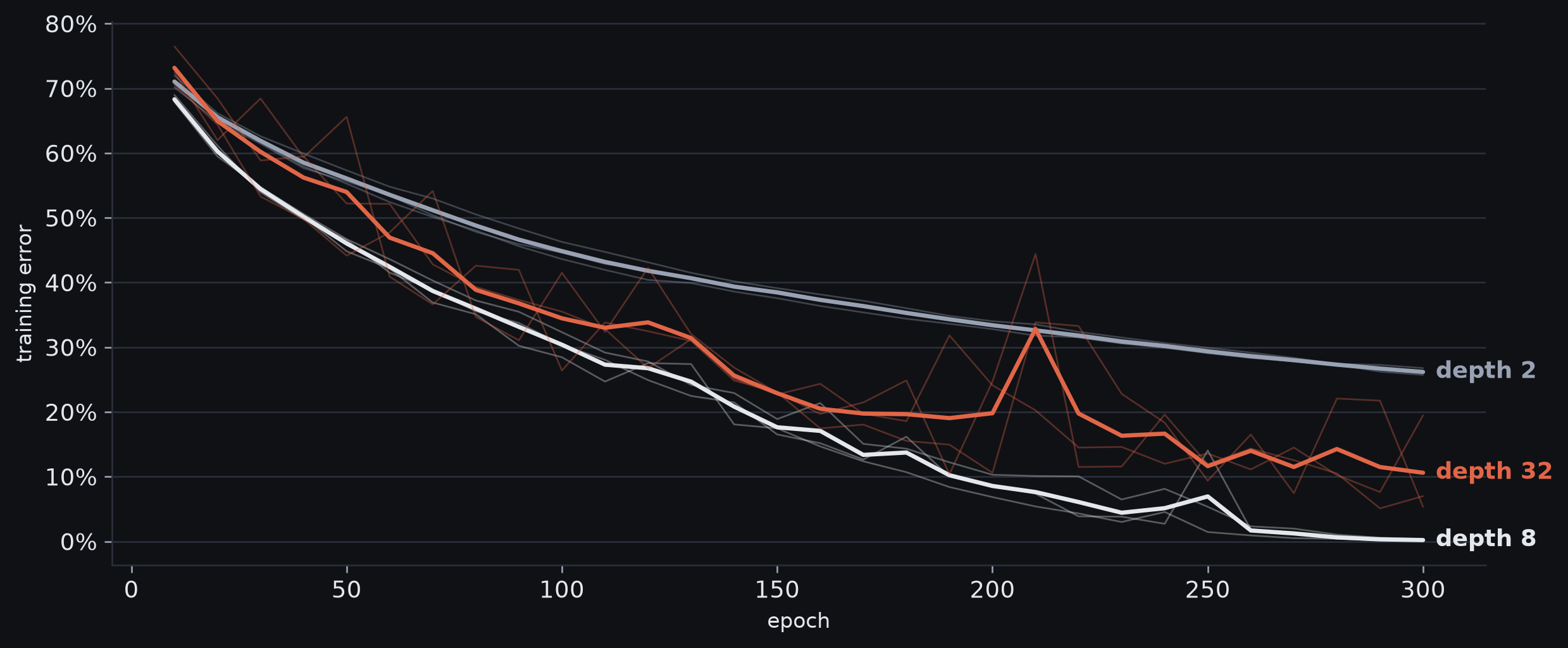
Training error on MNIST-1D for plain fully connected networks of depth 2, 8 and 32, counting hidden 64-to-64 layers: width 64, SGD at learning rate 0.005, three seeds each, faint lines for single runs, solid lines their mean.
The degradation problem
- Plain fully connected networks on MNIST-1D: width 64, the same optimiser, learning rate and epochs
- After 300 epochs, depth 8 ends at 0.2% training error; depth 32 ends at 10.6%
- every depth-32 run is worse than every depth-8 run: 5.4%, 19.5%, 7.0%
- the depth-32 runs are erratic, swinging by up to 33 points between checkpoints, so each end point is one snapshot
- depth 2 is worse still, and still falling at the end
- One shared learning rate and budget: evidence about this setup, not every setup
- The deeper network has more capacity, yet fits the training set worse: the degradation problem
- Overfitting usually appears as a growing train–test gap while training fit keeps improving
- Here the training fit itself gets worse with depth: this points to an optimisation problem
- The question: how do we make extra depth easy to optimise, and not just possible to represent?
Sequential networks
\[ \hidden_1=\vect{f}_1[\vect{x},\params_1],\qquad \hidden_2=\vect{f}_2[\hidden_1,\params_2],\qquad \hidden_3=\vect{f}_3[\hidden_2,\params_3],\qquad \vect{y}=\vect{f}_4[\hidden_3,\params_4] \]
- Each hidden \(\vect{f}_k\) is a complete layer transformation: an affine map followed by an activation, \(\vactivation{\layerbias+\layerweights\hidden_{k-1}}\); the last layer is usually affine alone
- Every route from input to output passes through every transformation
- A change in an early layer changes the input to every later layer
The chain rule through depth
- Each derivative says how one quantity responds to a small change in another
- Composing functions multiplies those local sensitivities
- For a scalar chain
\[ \frac{\partial y}{\partial h_1} = \frac{\partial h_2}{\partial h_1} \frac{\partial h_3}{\partial h_2} \frac{\partial y}{\partial h_3} \]
- A long chain makes the gradient depend on many successive transformations
Gradient steps
- A gradient describes an infinitesimal direction of change
- Gradient descent moves the parameters a finite amount
\[ \params \leftarrow \params-\alpha\nabla_{\params}\loss \]
- \(\alpha\): the learning rate
- The update lands at a different point on the loss surface
- Training is easier when the gradient there still resembles the old one
Shattered gradients
- Measure a scalar network’s sensitivity \(\partial y/\partial x\) while slowly changing the input \(x\)
- Autocorrelation at distance \(\Delta\): the correlation between \(\partial y/\partial x\) at \(x\) and at \(x+\Delta\), over all \(x\)
- shallow network: nearby inputs keep similar gradients over a wide range of \(\Delta\)
- deep plain network: the correlation falls off much faster with distance
- This fast loss of correlation is called shattered gradients
- Status: an observed phenomenon and a proposed explanation, not a theorem about every deep plain network
Gradients along the input
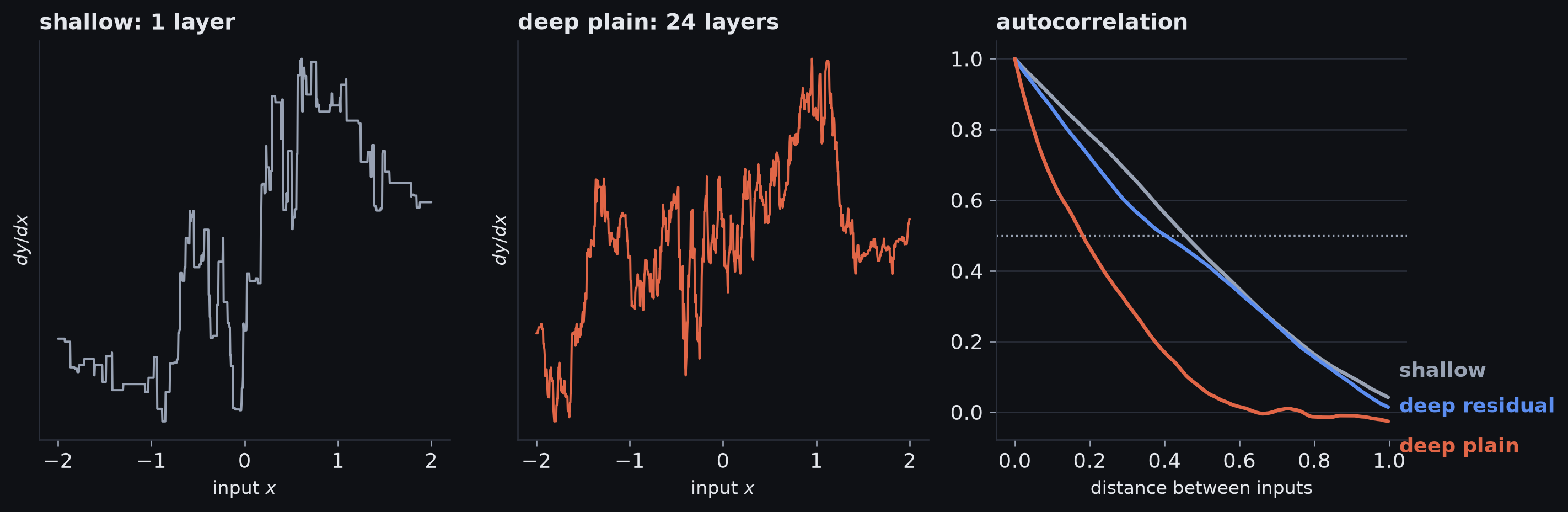
Width 200, with weights and biases drawn at variance 1/fan-in. Left and centre: dy/dx across the input for one shallow and one 24-layer plain network, each on its own vertical scale. Right: autocorrelation against input distance, averaged over twenty networks, with a 24-layer residual network whose branches are scaled by 1/sqrt(24); dotted line, one half.
Reading the autocorrelation
- Averaged over these 20 networks, correlation drops below one half at distance 0.46 for the shallow network and 0.18 for the deep plain one
- The scaled residual network sits between, nearer the shallow one, at 0.40
- One input, one output, at initialisation: a measurement of this setup, not a universal law
- The effect is sensitive to initialisation scale: using variance \(1/200\) in the input layer moves the deep network’s half-correlation distance to 0.31
- the deep network still decorrelates faster than the shallow one, but by less
Shattered gradients and gradient steps
- A gradient is local information: a finite step is useful only while that direction remains informative
- If nearby gradients change abruptly, a step can leave the region where the old gradient was a good guide
- The figure varies the input; optimisation moves the parameters
- input-gradient shattering does not by itself prove the same behaviour in parameter space
- treat it as evidence for a mechanism, not a direct measurement of the optimiser’s path
- Depth can therefore make the loss surface harder to navigate
Residual connections
Residual connections
- A plain layer replaces its input
\[ \hidden_{\text{out}} = \vect{f}[\hidden_{\text{in}},\params] \]
- A residual block adds a learned change to it instead
\[ \hidden_{\text{out}} = \hidden_{\text{in}} + \vect{f}[\hidden_{\text{in}},\params] \]
- The direct path from \(\hidden_{\text{in}}\) to \(\hidden_{\text{out}}\) is the skip, shortcut or identity connection
- \(\vect{f}[\hidden_{\text{in}},\params]\) is the residual branch: it learns the correction added to the stream
Identity as the default
- Suppose the best thing for a block to do is almost nothing
- a plain block must learn \(\vect{f}[\hidden]\approx \hidden\)
- a residual block only needs \(\vect{f}[\hidden]\approx \vect{0}\)
- The residual target is plausibly the easier one to reach: a hypothesis, not a theorem
- Residual: a branch is exactly \(\vect{0}\) whenever its last layer’s weights and bias are zero
- whatever the earlier layers are: the target sits at the origin of one layer’s weights, near where small initialisations start
- Plain: \(\relu(\mat{I}\hidden+\vect{0})=\hidden\) only because \(\hidden\ge\vect{0}\), the previous ReLU’s output
- the layers must undo each other exactly: \(\layerweights=\mat{I}\), or a later layer inverting an earlier one
- representable, but specific, structured weights far from a random draw
- Weight decay, from week 4, pulls weights towards zero: towards the residual target, away from the plain one
Reading the residual update
\[ \hidden_k=\hidden_{k-1}+\vect{f}_k[\hidden_{k-1},\params_k] \]
- \(\hidden_{k-1}\): the representation we already have
- \(\vect{f}_k[\hidden_{k-1},\params_k]\): the change block \(k\) proposes
- \(\hidden_k\): the updated representation
- Block \(k\) reads \(\hidden_{k-1}\); write \(\hidden_0=\vect{x}\)
- \(\vect{f}_k\) is the residual branch: it proposes a correction to the representation already on the stream
Matching shapes
- Addition needs both tensors to have the same shape
- If \(\hidden_{k-1}\in\reals^{C\times H\times W}\), the branch must return \(\vect{f}_k[\hidden_{k-1}]\in\reals^{C\times H\times W}\)
- If the spatial size or channel count changes, the skip path needs a matching projection
A residual block
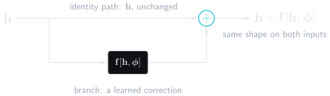
A residual block. The input travels unchanged along the identity path while the branch computes a learned correction; the two are added elementwise, so they must have the same shape.
Two paths through a block
- Identity path: carries \(\hidden\) directly
- Branch: computes \(\vect{f}[\hidden,\params]\)
- Merge: adds the two tensors
- The identity path crosses the block through no learned transformation at all
- The sequence \(\hidden_0,\hidden_1,\ldots\) carried along the identity paths is the residual stream; each branch reads from it and adds back to it
Stacking blocks
- Two residual blocks
\[ \hidden_1=\vect{x}+\vect{f}_1[\vect{x}], \qquad \vect{y}=\hidden_1+\vect{f}_2[\hidden_1] \]
- Substitute the first into the second
\[ \vect{y}=\vect{x}+\vect{f}_1[\vect{x}]+\vect{f}_2\!\left[\vect{x}+\vect{f}_1[\vect{x}]\right] \]
- The output mixes contributions that pass through different numbers of learned transformations
Gradients through the identity
- For vectors, the derivative of \(\hidden_k\) with respect to \(\hidden_{k-1}\) is the Jacobian from week 2: a \(D\times D\) matrix of partial derivatives, with \(D\) the width of the stream
- row \(i\) holds the derivatives of output \(i\), so the chain rule puts the later block’s Jacobian on the left
- week 2 wrote this orientation \(\partial\vect{z}/\partial\params\transpose\); from here the fraction alone means the same matrix
- matrices don’t commute, so the order matters in a way it didn’t for scalars
- A residual block’s Jacobian has an identity term
\[ \frac{\partial \hidden_k}{\partial \hidden_{k-1}} = \mat{I} + \frac{\partial \vect{f}_k}{\partial \hidden_{k-1}} = \mat{I}+\mat{J}_k \tag{1}\]
- \(\mat{I}\): direct sensitivity through the skip connection
- \(\mat{J}_k\): sensitivity through the learned branch
Expanding the product
- Two blocks: \(\partial\hidden_2/\partial\hidden_0\) is the later Jacobian times the earlier one
\[ (\mat{I}+\mat{J}_2)(\mat{I}+\mat{J}_1) = \mat{I}+\mat{J}_1+\mat{J}_2+\mat{J}_2\mat{J}_1 \]
- One term per route through the branches
- \(\mat{I}\): skips both
- \(\mat{J}_1\), \(\mat{J}_2\): passes through one branch
- \(\mat{J}_2\mat{J}_1\): passes through both
- TRY: expand \((\mat{I}+\mat{J}_3)(\mat{I}+\mat{J}_2)(\mat{I}+\mat{J}_1)\). How many terms pass through exactly one branch? Exactly two?
- \(K\) blocks: the product of the \(K\) factors expands into \(2^K\) terms
- \(\binom{K}{m}\), read “\(K\) choose \(m\)”, of them pass through exactly \(m\) branches: pick which \(m\) of the \(K\) blocks take the branch
Paths through two blocks
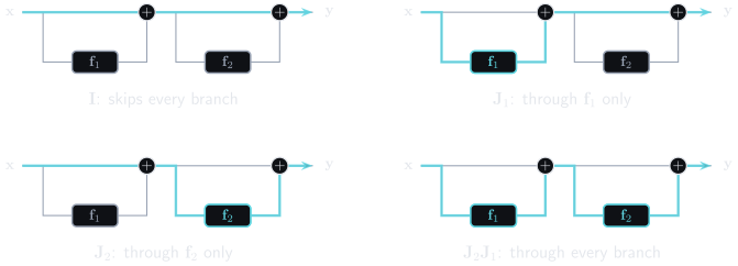
The same two-block residual network drawn four times, one route through it highlighted in each: one panel per term of the expanded product. A path through a branch picks up that branch’s Jacobian; the later branch’s sits on the left.
Unravelled paths
- Each term of the expansion is a path, one panel of the figure: at every block it either skips the branch or goes through it
- In the gradient the decomposition is exact
- In the forward pass the branches are nonlinear, so the \(2^K\) paths are a way of reading the network, not a literal sum
- The identity term reaches the early layers without passing through any branch
- gradients still arrive when the branch Jacobians are small or uninformative
- so shorter gradient paths exist, and shattered gradients are less severe: the scaled residual curve in the shattered-gradients figure
Path lengths
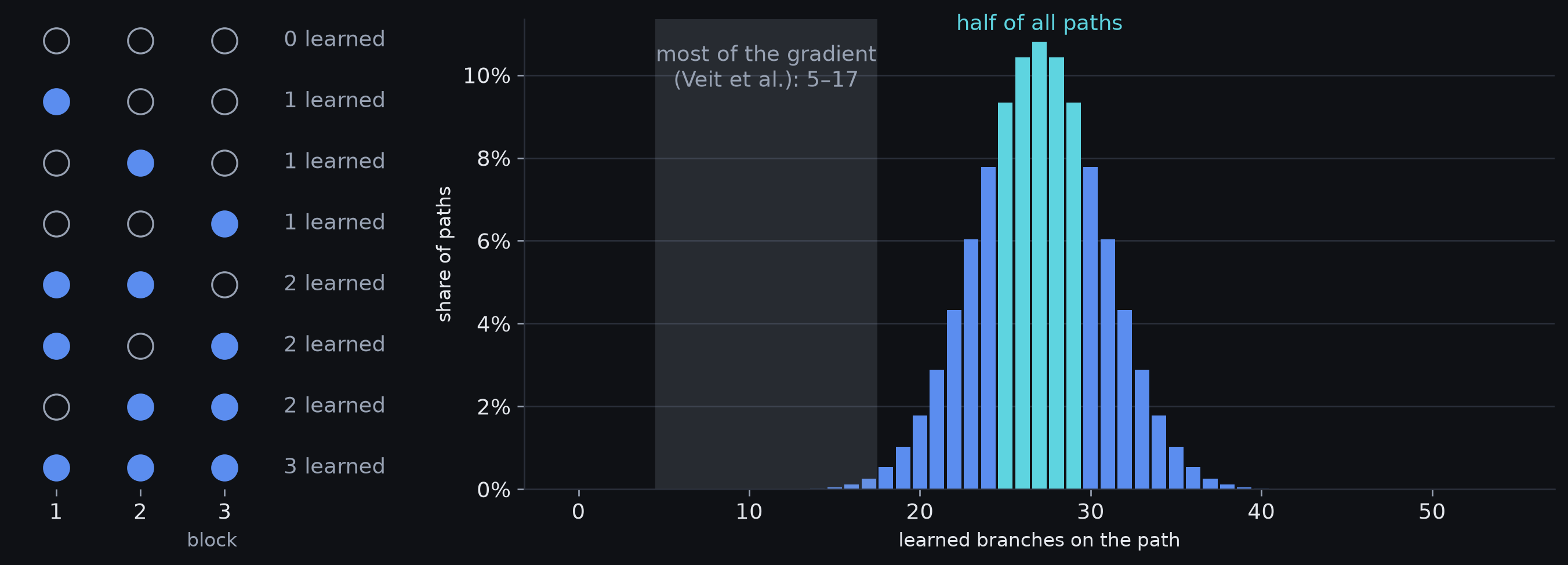
Left: the eight paths through three residual blocks, one row each, a filled dot where the path takes the learned branch. Right: for a network of 54 blocks, the share of its paths passing through each number of branches, with the central band holding half of all paths highlighted and, shaded, the lengths Veit et al. found carry most of the gradient.
Reading the path lengths
- Path counts follow \(\binom{54}{m}\): most combinatorial paths pass through an intermediate number of learned branches
- Counting paths is not the same as measuring how much gradient each path carries
- Veit et al. found that most gradient in their deep ResNet travelled through much shorter effective paths than the full network depth
- The useful conclusion is qualitative: residual networks provide many short routes for information and gradients
- Do not read the network as a literal ensemble of \(2^K\) independent forward models; the exact path expansion is a statement about the gradient product
Gradient scale through depth
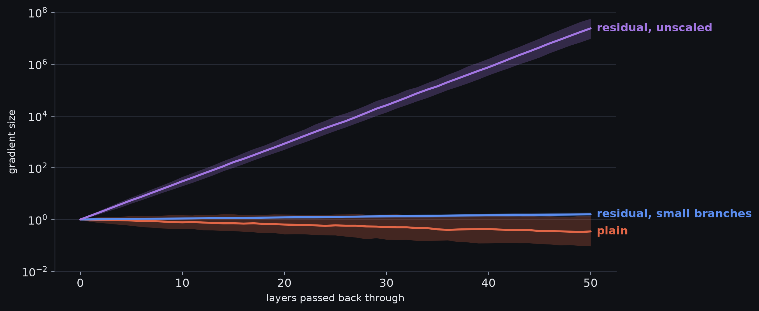
The size of a gradient with respect to the activations, after passing back through k layers from size 1, over 200 draws. Plain: a product of k random ReLU-layer Jacobians J. Residual: a product of I + J, or of I + J/sqrt(50) for small branches. The line is the median; the band runs from the 10th to the 90th percentile.
Reading the gradient scale
- Plain: multiplying many learned Jacobians can shrink a typical gradient and make its scale highly variable across draws
- Residual, unscaled: the identity term prevents pure multiplication by \(\mat{J}_k\), but repeated \(\mat{I}+\mat{J}_k\) factors can instead make gradients grow
- Residual, small branches: scaling each branch by \(1/\sqrt{K}\) keeps every update close to the identity and the gradient scale much more stable
- Residual connections solve neither vanishing nor exploding gradients automatically; the branch scale matters
Building residual blocks
Post-activation and pre-activation blocks
- A residual block has two jobs
- transform the residual branch
- preserve a clean shortcut path
- In the original post-activation ResNet block, the addition is followed by a ReLU
- the shortcut is simple, but the block output is still passed through a nonlinearity
- In a pre-activation block, normalisation and ReLU move before the weight layers in the residual branch
- the addition itself is left unobstructed
- successive blocks can therefore share a cleaner identity path
Why pre-activation helps
- The shortcut should be able to carry \(\hidden\) forward without forcing it through another learned transformation
- Pre-activation keeps BatchNorm and ReLU on the residual branch rather than after the merge
- The residual branch can still learn positive or negative corrections because its final operation is linear or convolutional
- “Pre-activation” here refers to the ordering of normalisation/activation before a weight layer inside the residual block
The initial projection
- Raw input does not yet live in the feature space used by the residual stream
- An initial linear or convolutional stem creates that representation
- sets the channel width expected by the residual blocks
- may also change spatial resolution in a CNN
- Residual blocks then refine an existing feature representation instead of repeatedly rebuilding it from raw input
Multi-layer branches
- A residual branch can contain several layers
- A typical branch
\[ \hidden \rightarrow \text{normalisation} \rightarrow \text{ReLU} \rightarrow \text{conv} \rightarrow \text{normalisation} \rightarrow \text{ReLU} \rightarrow \text{conv} \]
- Then add the original \(\hidden\)
- The block is residual; the branch can itself be a small network
- Normalisation controls the branch scale
Variance growth
Variance at initialisation
- He initialisation, from week 3, chooses weight scale to keep ReLU signal magnitudes from systematically exploding or collapsing through depth
- Work per component: \(h\) is one entry of \(\hidden_{k-1}\), and \(f[h]\) the matching entry of \(\vect{f}_k[\hidden_{k-1}]\)
- variances are over random inputs and a random draw of the weights
- Suppose a residual branch preserves variance: \(\var{f[h]}\approx \var{h}\)
- TRY: what is \(\var{h+f[h]}\)?
Variance of a sum
- For random variables \(A\) and \(B\)
\[ \var{A+B} = \var{A}+\var{B}+2\operatorname{Cov}\!\left[A,B\right] \]
- \(\operatorname{Cov}[A,B]=\expect{(A-\expect{A})(B-\expect{B})}\), read “the covariance of \(A\) and \(B\)”: zero when they don’t move together
- independence gives zero covariance; zero covariance doesn’t give independence
- If \(A\) and \(B\) are roughly uncorrelated
\[ \var{A+B} \approx \var{A}+\var{B} \]
Doubling per block
- At initialisation, \(\var{h}=v\)
- By the branch’s variance-preserving assumption, \(\var{f[h]}\approx v\)
- The branch’s last weights are zero-mean and drawn independently of \(h\)
- each term \(w_j g_j\) of \(f[h]\) carries a weight \(w_j\) with \(\expect{w_j}=0\), independent of \(h\), so \(\operatorname{Cov}[h,w_jg_j]=\expect{w_j}\expect{hg_j}-\expect{h}\expect{w_j}\expect{g_j}=0\)
- uncorrelated, though not independent: \(f[h]\) is still a function of \(h\)
\[ \var{h+f[h]}\approx 2v \]
- A stable branch plus a stable identity path does not make a stable sum.
Exponential growth
- If every block doubles the variance
\[ v_0=v,\qquad v_1\approx 2v,\qquad v_2\approx 4v,\qquad\cdots,\qquad v_K\approx 2^K v \]
- Residual connections ease one optimisation problem and create a forward-scale problem
- The same compounding runs backwards: each block can double the gradient’s expected squared size
Rescaling
- If a block doubles the variance, multiply its output by \(1/\sqrt{2}\)
\[ \var{\frac{h+f[h]}{\sqrt{2}}} \approx \frac{2v}{2}=v \]
- It preserves the expected variance under these assumptions
- a finite network can still wander because each block’s realised variance differs from its expectation
- Balduzzi et al. argue this controls gradient explosion but does not by itself resolve shattered gradients
- In practice, residual networks are more often stabilised by normalisation or careful branch scaling
We need to control scale without losing the shortcut
- The identity path fixes one optimisation problem: information and gradients no longer have to pass through every learned transformation
- But adding a full-sized residual branch at every block can make activation and gradient scales grow rapidly
- We want to keep the shortcut intact while making each residual branch operate at a controlled scale
- Batch normalisation is one historically important way to do that; careful residual scaling is another
Batch normalisation
Normalising over a batch
- One hidden unit produces scalar activations across a minibatch: \(\{h_i\}_{i\in\set{B}}\)
- Batch normalisation, or BatchNorm, uses the minibatch to ask
- where are these activations centred?
- how spread out are they?
- Then it standardises them and learns a new scale and offset
Step 1: batch mean
- For a minibatch \(\set{B}\) of \(|\set{B}|\) examples
\[ m_h=\frac{1}{|\set{B}|}\sum_{i\in\set{B}}h_i \]
- \(h_i\): the activation for example \(i\)
- \(m_h\): the batch mean, a statistic of the current minibatch and not a learned parameter
Step 2: batch spread
- Minibatch variance, in population form (divide by \(|\set{B}|\), not \(|\set{B}|-1\)), and standard deviation
\[ s_h^2=\frac{1}{|\set{B}|}\sum_{i\in\set{B}}(h_i-m_h)^2, \qquad s_h=\sqrt{s_h^2} \]
- The spread lets large activations be rescaled to a predictable range
Step 3: standardise
- Standardise each activation using the minibatch mean and variance
\[ \hat h_i= \frac{h_i-m_h}{\sqrt{s_h^2+\epsilon}} \]
- Subtracting \(m_h\) centres the batch on zero
- Dividing by the standard deviation gives variance near one
- \(\epsilon>0\) keeps the denominator numerically safe when the batch spread is tiny
Step 4: learned scale and offset
- Standardising alone would force every unit to mean zero and variance one
- BatchNorm then applies a learned scale and offset
\[ \tilde h_i=\gamma \hat h_i+\delta \]
- \(\gamma\): learned scale, initialised to 1
- \(\delta\): learned offset, initialised to 0
- so at the start BatchNorm is pure standardisation, and training can move each unit away from it
- Normalisation gives a controlled starting scale; \(\gamma\) and \(\delta\) restore the freedom to learn a different scale and centre
Worked example: four values
- TRY: one hidden unit over a minibatch, \([2,4,6,8]\), with \(\gamma=2\) and \(\delta=1\), taking \(\epsilon=0\)
- Mean: \(m_h=5\)
- Centred values: \([-3,-1,1,3]\)
- Population variance \(5\), so divide by \(\sqrt{5}\): \([-1.34,-0.45,0.45,1.34]\)
- Scale and shift: \([-1.68,0.11,1.89,3.68]\)
- Common slip:
torch.vardefaults to the unbiased form, \(6.67\) here; BatchNorm normalises with the population form
Four values, stage by stage
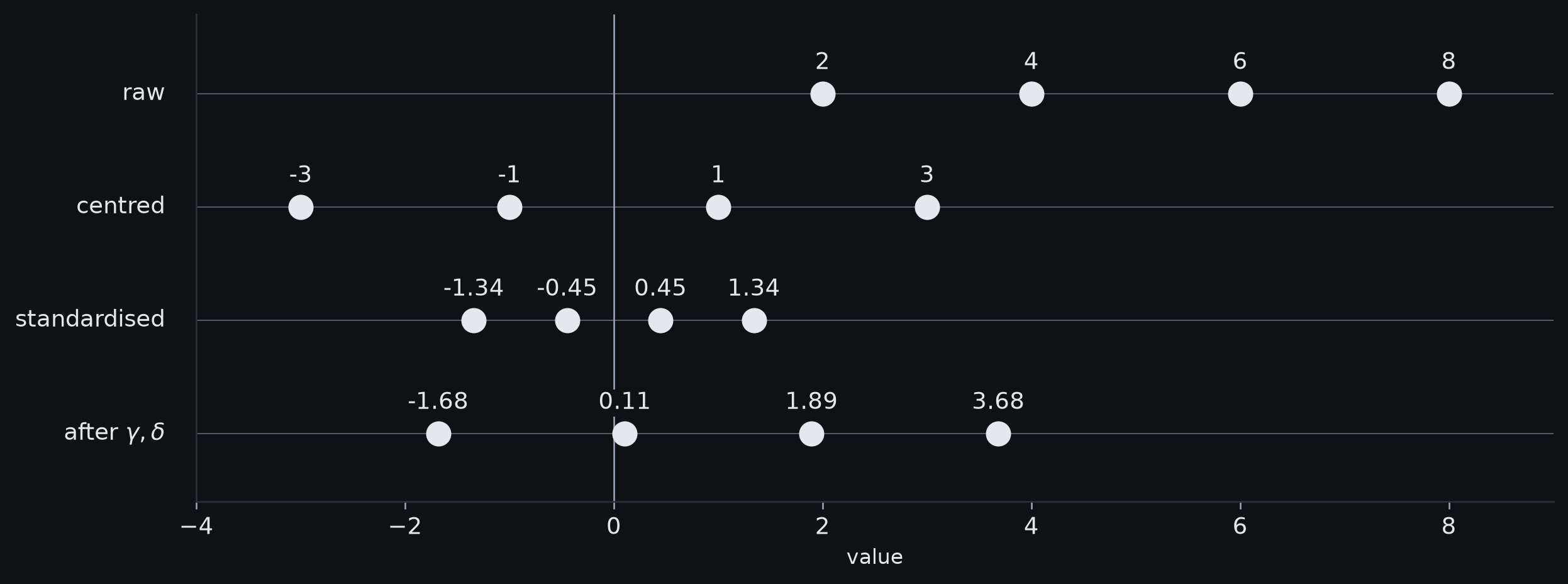
The four activations at each stage of batch normalisation, epsilon taken as zero. Centring moves their mean to zero; standardising scales their spread to one; the learned scale and offset then move them to wherever training prefers.
Per-feature statistics
- Fully connected layer with \(D\) hidden units
- each unit gets its own batch statistics
- each unit gets its own \(\gamma\) and \(\delta\)
- Convolutional activations of shape \((B,C,H,W)\)
- statistics per channel, over the batch and spatial positions
- each channel has its own \(\gamma\) and \(\delta\)
Training and inference
- Training: statistics from the current minibatch
- Inference: a single example may arrive with no meaningful batch
- so implementations use running estimates: moving averages of the batch mean and variance gathered during training, updated at every step
- normalising uses the population variance; PyTorch’s stored running variance uses the unbiased form
- Evaluation must run in inference mode; the implementation section shows the switch and the update
Linear variance growth
- Put BatchNorm at the start of each residual branch
- it strips the scale the stream has accumulated, so the branch input has variance one whatever \(k\) is
- He initialisation then gives a branch output of variance about one
- with \(\gamma=1\), \(\delta=0\) at initialisation, and the branch uncorrelated with the stream as before, the variances add
- With \(v_k=\var{h}\) after block \(k\)
\[ v_{k+1}\approx v_k+1 \quad\Longrightarrow\quad v_K\approx v_0+K, \qquad\text{against}\qquad v_K\approx 2^K v_0 \]
- So the total grows like \(O(K)\) rather than \(O(2^K)\)
- The important change is from exponential growth to roughly linear growth under this simplified initialisation model
Variance through depth
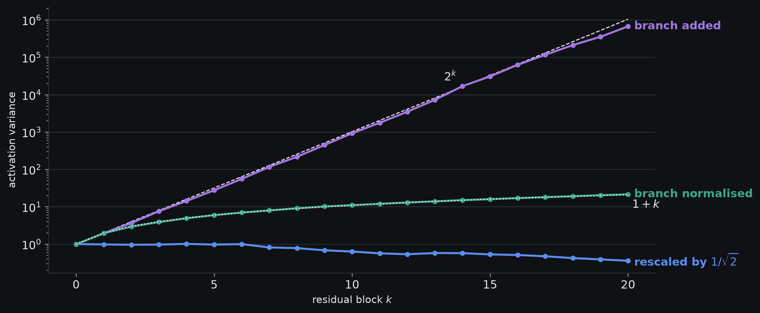
Activation variance after each of 20 residual blocks at initialisation, one random network of width 256 per curve, measured on a batch of 512 random inputs, on a log scale. Dashed: 2^k. Dotted: 1 + k, which the normalised curve lies on. The normalised branch batch-normalises its input, the block the depth-32 runs train.
Reading the variance curves
- Branch added: about 673,000 in this network after 20 blocks, against \(2^{20}=1{,}048{,}576\)
- Rescaled by \(1/\sqrt{2}\): stays within a small factor; this network wanders to 0.36, and other draws wander up
- each block’s variance ratio is random in a finite network, and the errors compound
- Branch normalised: 21.6 after 20 blocks, against \(1+20\)
- on the log axis this curve bends over, but it grows by about one per block: linear, not flat
Training at depth 32
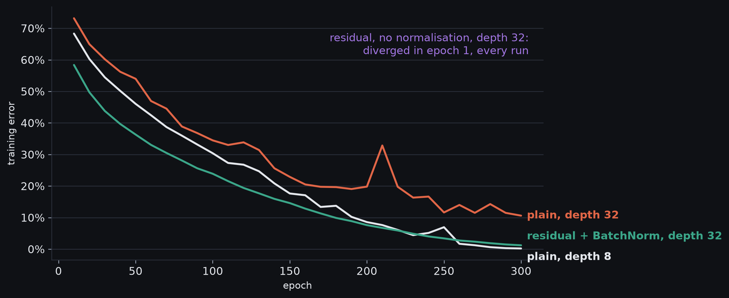
The MNIST-1D runs again: plain depth 8 and 32, and a depth-32 residual network with BatchNorm at the start of each branch. Lines are means over three seeds, at the same learning rate and epochs as before.
Reading the depth-32 runs
- Final training error: plain depth 8 0.2%, plain depth 32 10.6%, residual + BatchNorm depth 32 1.2%
- Residual + BatchNorm at depth 32 fits faster than plain depth 8 for most of training; plain depth 8 leads for good only from epoch 260
- The degradation gap at depth 32 falls from 10.4 to 1.0 points, but doesn’t close in this budget
- Without normalisation the residual network diverges in epoch 1 of every run, at learning rate 0.005
- its activation variance at initialisation grows like \(2^K\)
- no smaller learning rate was tried, so the runs don’t separate a too-large step from an unusable forward pass
- The comparison has no plain + BatchNorm run, so it doesn’t separate the skip connection’s contribution from BatchNorm’s
Relative size of later branches
- Suppose the residual stream has accumulated variance of order \(k\)
- The next normalised branch adds variance of order \(1\)
- So its relative contribution shrinks for later blocks
- At initialisation, a deep residual network behaves like a shallower one making many small corrections
- Training can then grow the learned scales and make those blocks matter more
BatchNorm and the loss surface
- Santurkar et al. found BatchNorm can make
- the loss vary more smoothly along optimisation directions
- gradients change more gradually
- larger learning rates practical
- Caveat: the exact mechanism isn’t settled
- Internal covariate shift: the change in a layer’s input distribution as earlier layers update
- BatchNorm’s original rationale was to reduce it, by fixing each unit’s batch mean and variance
- Santurkar et al. added noise after each BatchNorm layer to inject covariate shift, and it trained about as well as standard BatchNorm: evidence against that rationale
Batch noise
- The same example is normalised differently depending on which examples share its minibatch
- So BatchNorm is stochastic during training
- That noise can regularise, like other training-time noise
- It’s a side effect of batch statistics
One example in many batches
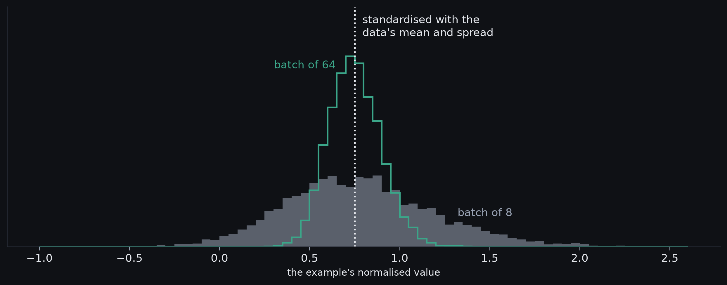
One example’s BatchNorm output, epsilon taken as zero, in 4,000 random minibatches of 8 and of 64. The unit’s activations over the data have mean 1 and standard deviation 2, and the example’s is 2.5. The dotted vertical line is the value standardising with the data’s own mean and standard deviation would give.
Reading the batch noise
- Same example, same weights: only its batch neighbours change
- Its normalised value centres near 0.75, the value the data’s own mean and spread give
- The spread across batches: standard deviation 0.42 with 8 examples, 0.14 with 64
- 3.0 times narrower for 8 times the batch, roughly \(1/\sqrt{|\set{B}|}\): the batch mean and spread are both averages over \(|\set{B}|\) draws
- Small batches make the noise larger, and the statistics less trustworthy
Scale invariance
- Multiply every pre-normalisation activation in the batch by a positive constant \(a\): \(h_i'=ah_i\) for all \(i\in\set{B}\)
- for example, by scaling the weights of a layer whose output goes straight into BatchNorm, such as the first convolution in a pre-activation branch
- that layer’s bias doesn’t matter: BatchNorm subtracts any per-feature constant
- this argument applies to a weight layer whose output goes directly into BatchNorm; it does not apply unchanged across a residual addition
- The batch mean and standard deviation both scale by \(a\), so, ignoring \(\epsilon\),
\[ \frac{ah_i-am_h}{as_h} = \frac{h_i-m_h}{s_h} \]
- For a weight layer whose output goes directly into BatchNorm, in training mode and ignoring \(\epsilon\), this is scale invariance: scaling the weights by positive \(a\) leaves the loss unchanged, \(\loss[a\layerweights]=\loss[\layerweights]\)
- For a weight layer immediately followed by BatchNorm, in training mode and ignoring \(\epsilon\), only the direction of \(\layerweights\) affects this normalised computation; its length cancels
- Differentiate \(\loss[a\layerweights]=\loss[\layerweights]\) with respect to the weights: \(a\nabla\loss[a\layerweights]=\nabla\loss[\layerweights]\)
- so the gradient at \(a\layerweights\) is \(1/a\) times the gradient at \(\layerweights\): gradient size \(\propto 1/\|\layerweights\|\)
- With a fixed learning rate \(\alpha\), the step \(\alpha\nabla\loss\) has length \(\propto\alpha/\|\layerweights\|\)
- Differentiating \(\loss[a\layerweights]=\loss[\layerweights]\) in \(a\) at \(a=1\) gives \(\layerweights\cdot\nabla\loss=0\): every step is perpendicular to \(\layerweights\)
- to first order it only turns \(\layerweights\); a finite step also lengthens it, \(\|\layerweights-\alpha\nabla\loss\|^2=\|\layerweights\|^2+\alpha^2\|\nabla\loss\|^2\)
- Turning a vector of length \(\|\layerweights\|\) by a perpendicular step changes its direction by about step length \(/\,\|\layerweights\|\)
- so the rate at which the direction turns falls like \(\alpha/\|\layerweights\|^2\): larger weights turn more slowly
- Consequence: \(\|\layerweights\|^2\) acts like an inverse learning rate; without weight decay it grows step by step and the turning slows, and weight decay shrinks it again
Residual architectures
ResNet blocks
- A pre-activation ResNet block
- normalisation, ReLU, convolution
- normalisation, ReLU, convolution
- add the skip path
- The skip path carries the representation; the branch learns a correction
Channel projection by \(1\times1\) convolution
- Last week’s \(1\times1\) convolution: it mixes channels at each pixel and leaves neighbouring pixels unmixed
- At pixel \((i,j)\), with input \(\hidden_{ij}\in\reals^{C_i}\)
\[ \vect{z}_{ij}=\layerbias+\layerweights\transpose\hidden_{ij}, \qquad \layerweights\in\reals^{C_i\times C_o} \]
- \(\layerweights\) is \(C_i\times C_o\), as last week; the transpose makes it act on \(\hidden_{ij}\)
- It’s a fully connected layer applied at every pixel, so it can change the channel count cheaply
Bottleneck blocks
- A full \(3\times3\) convolution is expensive when there are many channels
- A bottleneck branch is \(1\times1\rightarrow3\times3\rightarrow1\times1\)
- first \(1\times1\): reduce the channels
- \(3\times3\): mix spatial information at the reduced width
- last \(1\times1\): restore the channel count
- The sum with the skip path works again once the branch’s shape matches
- TRY: count the weights, ignoring biases, in a basic branch (two \(3\times3\) convolutions, 256 to 256) and a bottleneck branch (256 to 64 to 64 to 256)
- from \(C_i\) to \(C_o\) channels, a \(3\times3\) convolution has \(9C_iC_o\) weights and a \(1\times1\) has \(C_iC_o\)
Weights in a bottleneck
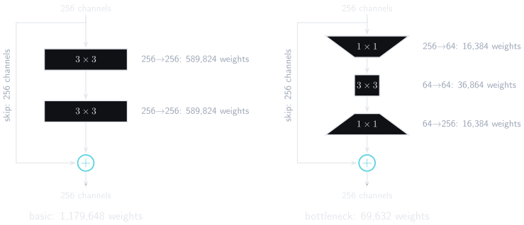
A basic block’s branch, left, and a bottleneck branch, right, each taking 256 channels back to 256. Each layer’s top and bottom edges widen with its input and output channels, and the skip path carries all 256 around the branch to the sum. Weights exclude biases.
Counting the bottleneck’s weights
- Basic: two \(3\times3\) layers at 256 channels, \(2\cdot 9\cdot 256^2=1{,}179{,}648\)
- Bottleneck: \(256\cdot64+9\cdot64^2+64\cdot256=69{,}632\)
- About \(1/17\) of the weights
- one \(3\times3\) layer at a quarter of the width costs \(1/32\) of the basic branch
- the two \(1\times1\) layers add almost as much again: 47% of the bottleneck’s weights
Downsampling stages
- A residual stage may change
- the spatial resolution
- the number of channels
- Then the old representation can’t be added to the new one directly
- Typical repairs
- a strided \(1\times1\) projection on the skip path
- padding or channel adjustment
- The identity idea survives, through a simple projection
DenseNet
- Residual addition: \(\hidden_k=\hidden_{k-1}+\vect{f}_k[\hidden_{k-1}]\)
- DenseNet concatenates instead
\[ \hidden_k=\operatorname{concat}\left(\hidden_{k-1},\vect{f}_k[\hidden_{k-1}]\right) \]
\(\hidden_{k-1}\) already holds the input and every earlier layer’s output, so each layer sees all of them
Addition keeps the width fixed; concatenation grows it
- each \(\vect{f}_k\) outputs a fixed number \(g\) of new channels, the growth rate, so layer \(k\) sees \(C_0+(k-1)g\)
TRY: \(C_0=64\), \(g=32\). How many channels enter layer 12?
Trade-offs of concatenation
- Dense connections give later layers direct access to earlier representations
- Benefits
- feature reuse
- short paths for information
- short paths for gradients
- Costs
- the channel count grows quickly
- later convolutions get expensive
- \(1\times1\) bottlenecks and stage boundaries control the growth
Width in a dense block
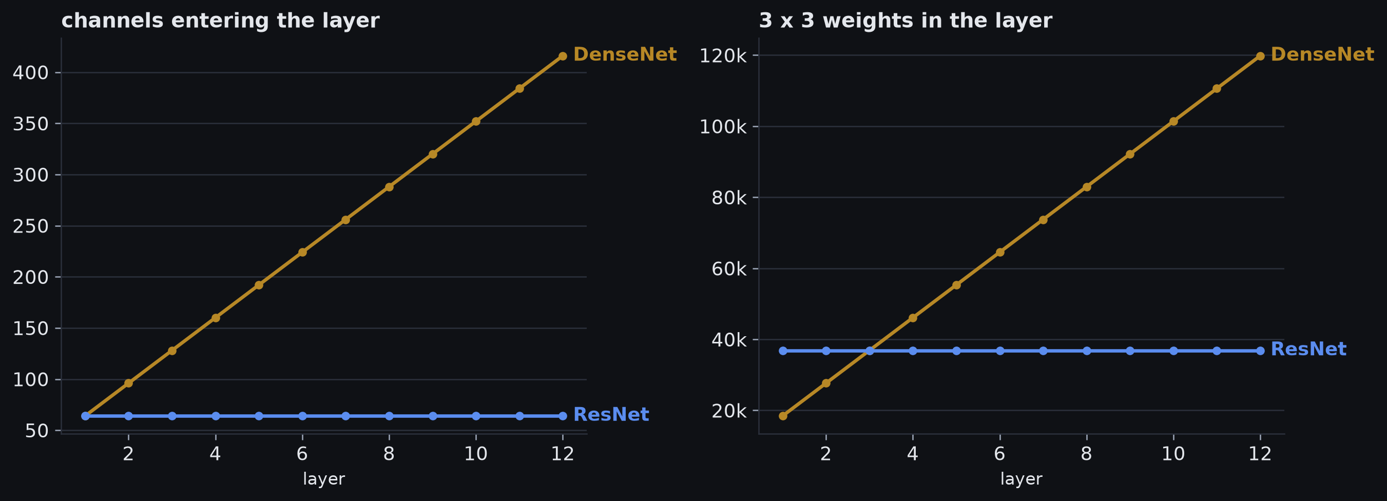
A dense block of 12 layers with growth rate 32, against a residual stage of constant width 64. Left: the channels entering each layer, which concatenation grows by 32 every layer. Right: the weights in that layer’s 3 x 3 convolution; each dense layer outputs 32 channels and each residual layer 64, so the dense layers start cheaper, draw level at layer 3 and cost more after.
Reading the dense block
- Channels entering layer 12: 416 for DenseNet, against 64 for the residual stage
- Weights in layer 12’s \(3\times3\) convolution: 119,808 against 36,864
- a dense layer’s cost grows with every earlier layer it reads
- This growth is why DenseNet adds \(1\times1\) bottlenecks and compresses width at stage boundaries
U-Net
- An encoder-decoder compresses an image to build large receptive fields
- Aggressive downsampling loses precise spatial detail
- U-Net sends high-resolution encoder features straight to the decoder stage of matching scale
- Here the skip mainly recovers spatial detail; the optimisation shortcut is only part of its role
Concatenation in U-Net
- At a matching spatial scale
\[ \hidden_{\text{decoder}}'= \operatorname{concat} \left(\hidden_{\text{decoder}},\hidden_{\text{encoder}}\right) \]
- Decoder features: coarse semantic context
- Encoder features: fine spatial information
- Later convolutions learn how to combine the two
U-Net skips
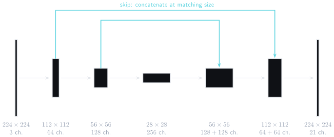
Last week’s encoder-decoder shapes, with U-Net’s skips added; box height is spatial size and box width is channels. Each intermediate encoder stage’s features are carried across and concatenated with the decoder stage of the same spatial size, which widens it, returning detail at the 112 x 112 and 56 x 56 resolutions that the downsampling discarded.
Hourglass networks
- Hourglass models repeatedly
- downsample to integrate global context
- upsample to recover spatial precision
- pass skips between matching scales
- Unlike U-Net, each skip is processed by further convolutions and added, not concatenated
- Several hourglasses are often stacked
- Used for tasks such as human pose estimation, where the output is often one heatmap per joint
- The same principle, short routes around expensive transformations, serves a task-specific purpose
Normalisation choices
Limits of batch statistics
- Batch statistics are convenient when batches are large and representative
- They become awkward when
- batches are very small
- distributed workers see different fragments of a batch
- sequence lengths vary
- one example’s output shouldn’t depend on its batch neighbours
- Other schemes change which axes supply the statistics
Normalisation schemes
| Method | Statistics gathered across, for activations \((B,C,H,W)\) |
|---|---|
| BatchNorm | batch and spatial positions, separately per channel |
| LayerNorm | channels and spatial positions within each example |
| GroupNorm | groups of channels and spatial positions within each example |
| InstanceNorm | spatial positions within each channel and example |
- Each answers one question: which values define a typical centre and scale for this activation?
Normalisation axes
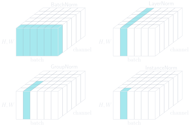
An activation tensor drawn with its batch, channel and spatial axes, one faint line per example and per channel, in the order of the table. The shaded values are the ones one mean and variance are computed over. BatchNorm: one channel across the batch and every position. LayerNorm: one example across every channel and position. GroupNorm: a group of channels of one example, across positions. InstanceNorm: one channel of one example.
BatchNorm and LayerNorm
- BatchNorm: how unusual is this channel value, relative to this minibatch?
- LayerNorm: how unusual is this feature value, relative to this example’s other features?
- So LayerNorm is easier to use when there’s no stable batch dimension
- Transformer blocks similarly combine residual streams with LayerNorm
- each token is normalised over its embedding features, not across the batch or across token positions
Residual networks without BatchNorm
- Other approaches control residual scale directly
- Rescale the sum: multiply \(\hidden+\vect{f}[\hidden]\) by \(1/\sqrt{2}\)
- Shrink the branch before adding it
- Stable ResNet: a fixed constant on the \(k\)th branch, such as \(1/\sqrt{K}\)
- SkipInit: a learned scalar on each branch, initialised to zero
- FixUp: the branch’s last layer initialised to zero
- The branch-shrinking methods start near the identity, \(\hidden_k\approx\hidden_{k-1}\); SkipInit and FixUp then let training grow each branch
Why residual networks work
Beyond depth
- Residual connections let us train networks with many more layers
- Depth alone doesn’t explain the gains
- wide residual networks can beat deeper, narrower ones (Zagoruyko and Komodakis)
- very long paths may contribute little gradient
- skip-connected loss surfaces can be smoother near solutions
- Residual connections change the optimisation geometry, not merely the number of layers
Direct and transformed information
\[ \hidden_k=\hidden_{k-1}+\vect{f}_k[\hidden_{k-1}] \]
- The shortcut preserves the representation already in \(\hidden_{k-1}\)
- The residual branch can add a learned transformation without forcing the block to rewrite the whole representation
Short paths
- Across the architectures in this chapter
- ResNet: identity paths around blocks
- DenseNet: concatenated access to earlier features
- U-Net: direct paths from encoder to decoder at each scale
- hourglass networks: shortcuts across scales and blocks
- All four architectures create shorter routes for earlier representations, but they use those routes for different purposes
Replace, add or concatenate
| Choice | Update | Earlier representation | Width |
|---|---|---|---|
| Replace | \(\hidden_k=\vect{f}_k[\hidden_{k-1}]\) | rewritten | set by \(\vect{f}_k\) |
| Add | \(\hidden_k=\hidden_{k-1}+\vect{f}_k[\hidden_{k-1}]\) | kept, mixed with the change | fixed |
| Concatenate | \(\hidden_k=\operatorname{concat}(\hidden_{k-1},\vect{f}_k[\hidden_{k-1}])\) | kept, as separate channels | grows |
Implementation
Residual addition in code
- The one-line addition carries a contract
- shapes must match, and PyTorch silently broadcasts shapes that differ in a size-1 or missing leading dimension, so assert it
- the branch output’s scale must stay manageable
- a projection on the skip path changes the exact identity
Train and eval modes
eval()does not mean “compute a validation score”; it changes how modules behave- Dropout is another layer the same switch affects
Running estimates
- Frameworks keep running estimates of the activation statistics during training and use them at inference
- Each step moves the estimate a fraction \(\rho\) towards the current batch: \(\bar m\leftarrow(1-\rho)\bar m+\rho\, m_h\), and the same for the variance
- PyTorch calls \(\rho\)
momentum; it’s unrelated to optimiser momentum
- PyTorch calls \(\rho\)
- So correctness depends on
- a sensible \(\rho\)
- enough representative training batches
- switching to evaluation mode for inference
Running estimates over training
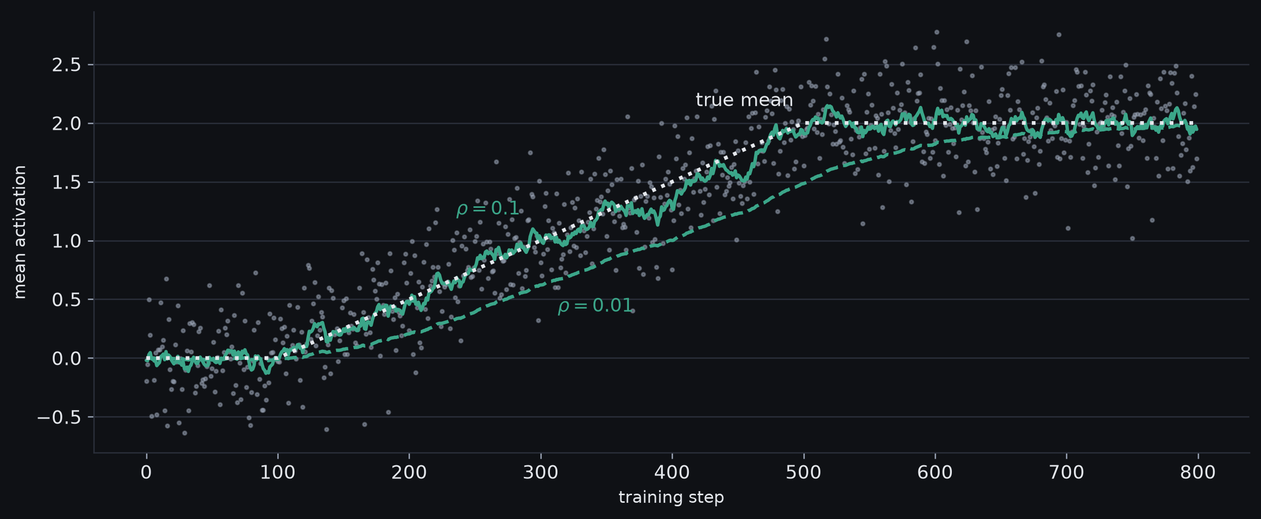
A synthetic unit whose true activation mean, dotted, drifts from 0 to 2 between steps 100 and 500 as training changes the weights. Dots: the batch mean at each step, noise standard deviation 0.3. Lines: running estimates starting at 0, at two values of rho.
Reading the running estimates
- A larger update rate \(\rho\) follows changing activation statistics more quickly, but the estimate is noisier
- A smaller \(\rho\) is smoother, but it can lag behind a network whose activations are still changing
eval()uses the stored estimates from training, so those estimates need enough representative batches to become useful- PyTorch calls \(\rho\)
momentum; it is unrelated to optimiser momentum
Projections on the skip path
- The projection exists to satisfy the addition contract
Revision
Degradation and overfitting
- TRY: error rises when depth goes from 8 to 32. What would you plot to tell overfitting from degradation, and what would each look like?
- Overfitting
- training fit continues to improve
- test performance eventually worsens, increasing the train–test gap
- Degradation in deep plain networks
- training performance worsens too
- a sign of an optimisation difficulty
Vanishing and shattered gradients
- Vanishing gradient: its size shrinks towards zero through depth
- Shattered gradient: nearby gradients become poorly correlated
- A gradient can have a reasonable size and still be a poor guide for a finite step
Skip connections and computation
- \(\hidden_k=\hidden_{k-1}+\vect{f}_k[\hidden_{k-1}]\)
- the skip path preserves \(\hidden_{k-1}\)
- the branch still computes a learned transformation
- the addition combines both
- The shortcut makes the transformation optional in effect; it is still computed
BatchNorm in four steps
- estimate the batch centre
- estimate the batch spread
- standardise
- learn a new scale and offset
- Training and inference use different statistics
Variance with BatchNorm
- In the simplified initialisation argument
- a normalised branch contributes controlled variance
- the residual stream still grows as branches are added
- the growth is roughly linear, not flat
- The assumptions are approximate; branch correlations and learned parameters matter in real networks
- TRY: \(v_0=1\). After three blocks, what is \(v_3\) with BatchNorm at the start of each branch? Without it?
- With it, \(v_3\approx 1+3=4\); without it, \(v_3\approx 2^3=8\)
- TRY: which week-3 argument does the doubling reuse?
- Week 3’s fan-in argument: independent contributions add on the variance scale; the sum rule needs only uncorrelated, which \(h\) and \(f[h]\) are
ResNet, DenseNet and U-Net skips
| ResNet | DenseNet | U-Net | |
|---|---|---|---|
| Merge | add | concatenate | concatenate |
| Earlier features | mixed with the new | kept as separate channels | carried past the coarsest stage |
| Width | fixed | grows unless controlled | grows at each merge |
| Main purpose | short optimisation path | feature reuse | restore spatial detail |
Summary
- Very deep plain networks can be harder to optimise, even on training data
- Residual blocks learn additive corrections around shortcut paths
- Identity shortcuts give information and gradients shorter routes
- Addition makes activation variance grow quickly with depth
- Normalisation or residual scaling controls that growth
- BatchNorm is also found to smooth optimisation, and it adds training noise
- ResNet, DenseNet and U-Net use shortcuts for different architectural goals
- Very deep residual models don’t rely only on their longest paths
Reading for Friday
- Prince, chapter 11, if not yet read
- Prince, sections 12.1–12.3: text as data, dot-product self-attention and its extensions
- Vaswani et al., Attention Is All You Need, in full (Vaswani et al. 2017)
- the paper writes \(\mat{Q}\mat{K}\transpose\) with one token per row; Prince puts tokens in columns, so its products appear transposed
- Reading the paper: you’re not expected to follow every line. Before Friday, be able to answer
- What question is the paper asking?
- What is the main claim?
- What experiment or argument supports it?
- Which figure or table carries the claim?
- What assumption seems most important?
- What did you not understand?
Source and revision locators
- Simon J. D. Prince, Understanding Deep Learning, Chapter 11: “Residual networks” (Prince 2023)
- Sections: 11.1 sequential processing and degradation; 11.2 residual connections and blocks; 11.3 exploding gradients; 11.4 batch normalisation; 11.5 ResNet, DenseNet, U-Net and hourglass networks; 11.6 why residual networks perform well; and the chapter notes
- Equations: 11.1–11.3 sequential chain and chain rule; 11.4–11.6 residual update and unravelled paths; 11.7–11.9 batch normalisation
- Figures worth revisiting: 11.4 unravelled paths; 11.5 block ordering; 11.6 variance growth; 11.7 ResNet and bottleneck blocks; 11.8 ResNet-200; 11.9–11.10 DenseNet and U-Net; 11.13 loss surfaces; 11.14 normalisation variants
- Notebooks: 11.1 shattered gradients; 11.2 residual networks; 11.3 batch normalisation
- Problems: 11.1–11.9