Lecture 8: Convolutional Networks
Week 4 · architectures
Images and dense layers
Image size
- A typical classification input is a \(224\times224\) RGB image
- Flattened, it is one vector of
\[ 224\times224\times3=150{,}528 \]
A dense hidden layer of the same width needs
\[ 150{,}528^2 \approx 2.27\times10^{10} \]
weights
Nothing in the layer’s structure encodes the fact that the input is an image.
Image geometry
- Adjacent pixels usually belong to related parts of the scene
- Flattened row by row, channels last, the pixel directly below \(x_i\) sits 672 positions away
- A dense layer can learn spatial relationships, but its connectivity gives nearby pixels no special status
- Reorder every image by the same fixed permutation and permute a dense layer’s weight columns the same way
- the images look scrambled
- the dense layer computes exactly the same outputs
- so training on scrambled images is the same problem: nothing in the architecture can exploit adjacency
- Images have local structure, so it is useful to privilege interactions between nearby values
Permuted pixels
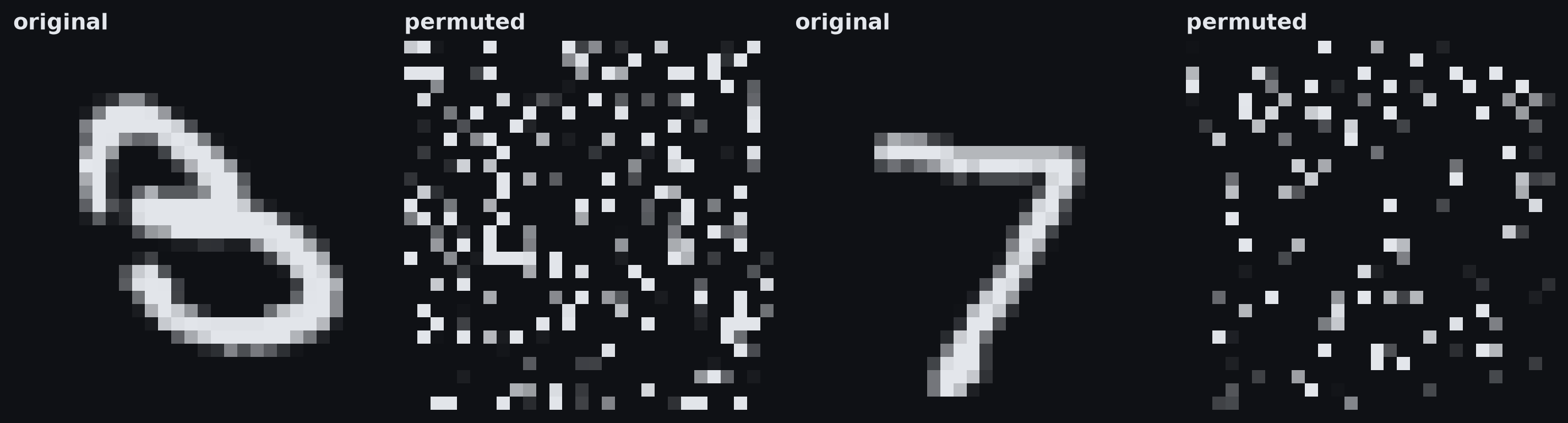
The same two digits before and after one fixed permutation of their 784 pixels. A dense layer whose weight columns are permuted the same way computes exactly the same outputs from the scrambled images, so nothing in its connectivity records which pixels were neighbours. MNIST, LeCun and Cortes, CC BY-SA 3.0.
Repeated patterns
- A small edge, corner, texture or object part can appear
- on the left or the right
- near the top or the bottom
- anywhere in between
- A dense layer gives each position its own weights
- Nothing ties those weights together, so a detector learned at one position doesn’t transfer to another
Dense and convolutional connectivity
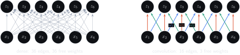
Left: a dense layer from six inputs to six outputs, one free weight per edge. Right: a convolution with kernel size three over the same units. Each output reads only its neighbours, and every edge of one colour carries the same weight. Inputs past the edge count as zero, so the end outputs lose the edge that would reach past the input.
- Compare the two panels
- Which edges share one parameter in the convolution?
- Which assumptions about the input differ?
Locality and weight sharing
- Locality: compute each output from a small neighbourhood
- Weight sharing: use the same local computation at every position
- Together they give
- far fewer trainable parameters
- an explicit notion of neighbourhood
- a shifted pattern gives the same response, shifted
Inductive bias
- Inductive bias, from last Friday: a learning system’s tendency to favour some solutions over others when the data don’t uniquely determine the function
- It can be a soft preference or a hard restriction
- Soft: the L2 penalty from Monday prefers small weights but forbids none
- Hard: weight sharing rules out any layer that applies different local weights at different positions
- For images, convolution restricts the model to functions that
- process local regions first
- reuse the same detector across positions
- keep spatial structure through intermediate representations
- The restriction helps generalisation when those assumptions match the data
Invariance and equivariance
Translation invariance
- Shift an image of a mountain 20 pixels right: the class is still mountain
- Write
- \(\vect{x}\) for an image
- \(\vect{t}[\vect{x}]\) for the translated image
- \(\vect{f}[\vect{x}]\) for the model’s output
- Translation invariance: the input moves, the output stays the same
\[ \vect{f}[\vect{t}[\vect{x}]] = \vect{f}[\vect{x}] \]
Definition 1 A model \(\vect{f}\) is translation invariant if translating its input leaves its output unchanged: \(\vect{f}[\vect{t}[\vect{x}]] = \vect{f}[\vect{x}]\) for every input \(\vect{x}\) and every translation \(\vect{t}\).
Translation equivariance
- In semantic segmentation the output is itself an image
- shift the cat in the input
- the predicted cat mask should shift by the same amount
- Translation equivariance: the input moves, the output moves with it
\[ \vect{f}[\vect{t}[\vect{x}]] = \vect{t}[\vect{f}[\vect{x}]] \]
Definition 2 A model \(\vect{f}\) is translation equivariant if translating its input translates its output in the same way: \(\vect{f}[\vect{t}[\vect{x}]] = \vect{t}[\vect{f}[\vect{x}]]\) for every input \(\vect{x}\) and every translation \(\vect{t}\).
A shifted pattern
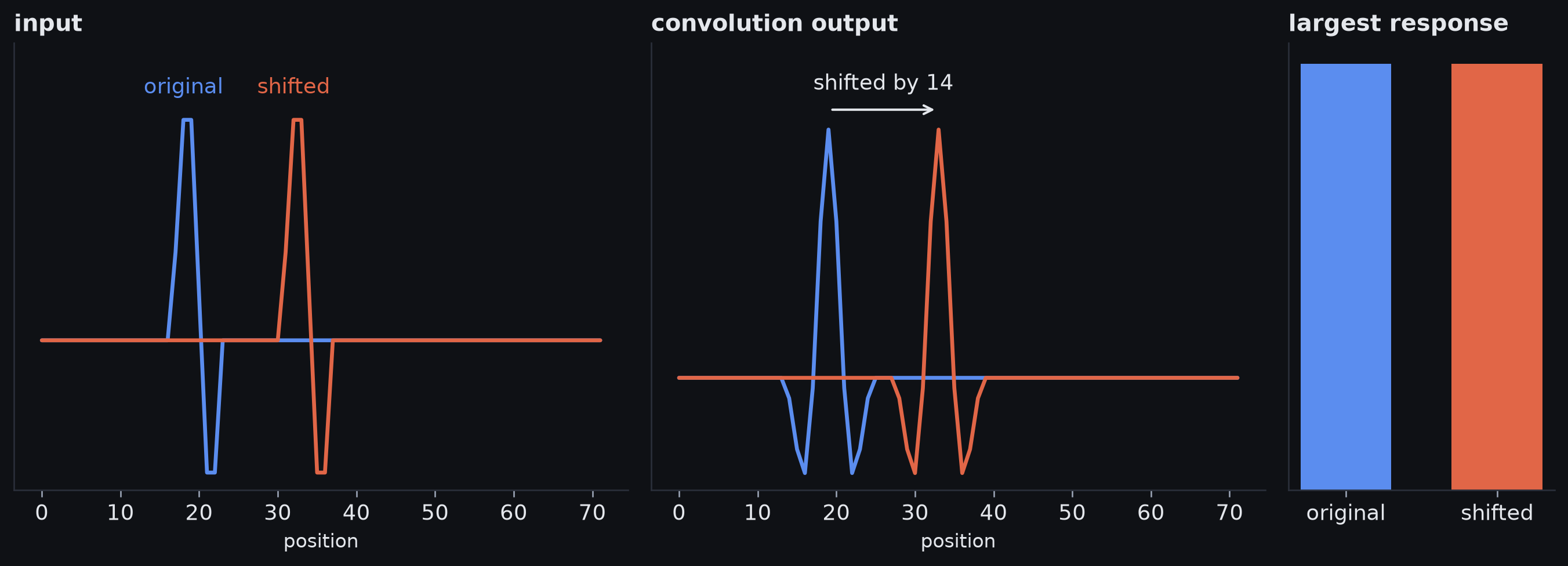
Left: a short pattern, and the same pattern shifted to the right. Centre: a convolution with a kernel matched to the pattern. Its response shifts by exactly the same amount, which is equivariance. Right: the largest response anywhere in the signal is the same for both, which is invariance.
Invariance and equivariance by task
| Task | Input | Desired output |
|---|---|---|
| Image classification | object moves | class stays the same |
| Semantic segmentation | object moves | mask moves with it |
| Keypoint localisation | object moves | keypoints move with it |
- Stride-1 convolutional layers are translation equivariant, away from the boundary
- stride: the step between neighbouring kernel positions
- Local pooling summarises each small block of a feature map, a layer’s output over positions, by one number, such as its maximum
- it discards some positional detail, so later representations are less sensitive to small shifts
- Global pooling summarises each channel, one feature map, by one number over all positions
- it removes position entirely, and can turn an equivariant feature map into an invariant summary
Equivariance in practice
- Ideal discrete convolution, away from boundaries and downsampling
- translating the input translates the output
- the same kernel, the shared local weights, is applied everywhere
- Real CNNs break exact equivariance in three places
- Padding: outputs near the edge read values invented beyond it
- Finite boundaries: content shifted past the edge is lost
- Stride and pooling: with step \(S\), for pooling its block size, an input shift of \(nS\) moves the output \(n\) positions, so equivariance holds only up to the change of grid
- A network’s total sampling step \(S_{\text{total}}=S_1S_2\cdots\) multiplies all its strides and pooling steps
- Ignoring boundary effects, it stays exactly equivariant only for shifts by multiples of \(S_{\text{total}}\)
Convolution in 1D
A local weighted sum
- Take a 1D signal \(\vect{x}=[x_1,x_2,\ldots,x_D]\transpose\)
- At position \(i\), read only the nearest three values: \(x_{i-1},\;x_i,\;x_{i+1}\)
- Weight them with three numbers, the same at every position: \(\kernel=[\omega_1,\omega_2,\omega_3]\transpose\)
- read \(\kernel\) as “bold omega”, the whole kernel; \(\omega_j\) is one of its numbers
Definition 3 A kernel, or filter, is the vector of weights \(\kernel=[\omega_1,\ldots,\omega_K]\transpose\) applied to every local window of the input. Each weight is one tap, and the number of taps \(K\) is the kernel size.
One output
- For kernel size \(3\), the output at position \(i\) is
\[ z_i = \omega_1x_{i-1}+\omega_2x_i+\omega_3x_{i+1} \]
- To compute it
- align the kernel with position \(i\)
- multiply corresponding values
- add the three products
- Each output is a dot product between the kernel and a local window.
An edge kernel
- Window: \([x_{i-1},x_i,x_{i+1}] = [2,5,4]\)
- Kernel: \(\kernel=[-1,0,1]\transpose\)
\[ z_i=(-1)(2)+(0)(5)+(1)(4)=2 \]
- Here \(z_i=x_{i+1}-x_{i-1}\)
- positive where the signal rises
- negative where it falls
- blind to the centre value \(x_i\)
The kernel at three positions
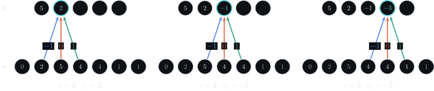
The kernel [-1, 0, 1] at three neighbouring positions of one signal. Each highlighted output has one connection from each input in its window, and the connections carry the kernel’s weights: the same three, in the same colours, in every panel. The output row fills in one value per position. Outputs exist only where the whole window fits, so none sits above the end inputs. The first panel is the worked example from the previous slide.
Weight sharing
\[ \begin{aligned} z_i &= \omega_1x_{i-1}+\omega_2x_i+\omega_3x_{i+1}\\ z_{i+1} &= \omega_1x_i+\omega_2x_{i+1}+\omega_3x_{i+2} \end{aligned} \]
- The input window changes
- The weights do not
- The same local question is asked at every position
- Weight sharing, with a fixed kernel size, makes the parameter count independent of signal length.
Convolution and cross-correlation
- Deep-learning libraries compute
\[ z_i = \sum_{j=1}^{3} \omega_j x_{i+j-2} \]
\(j=1,2,3\) reads \(x_{i-1},x_i,x_{i+1}\): the sum from the previous slides
Mathematical convolution flips one operand first; the unflipped operation is cross-correlation
\[ \text{convolution:}\quad z_i = \sum_{j=1}^{3} \omega_j x_{i-j+2} \]
- The flip only reverses the kernel to \([\omega_3,\omega_2,\omega_1]\), so a learned kernel loses nothing: the optimiser learns the reversed weights instead
- Convention: deep-learning APIs call cross-correlation “convolution”, and so do these slides
Equivariance of convolution
- Shift the input \(s\) positions right: \(x'_i=x_{i-s}\)
- Apply the same kernel to the shifted input
\[ \begin{aligned} z'_i &= \sum_{j=1}^{3}\omega_j x'_{i+j-2}\\ &= \sum_{j=1}^{3}\omega_j x_{(i-s)+j-2}\\ &= z_{i-s} \end{aligned} \]
- Line two substitutes the shift; line three is the original sum at position \(i-s\)
- Away from the edges, the response is the original response shifted \(s\) positions: convolution is translation equivariant.
- The detector needs no new parameters for the new position
Convolutional layers
Convolutional hidden unit
- A dense hidden unit: weighted sum, then bias, then activation
\[ h_i=\activation{\beta_i+\sum_{j=1}^{D}\omega_{ij}x_j} \]
- A convolutional unit keeps that recipe and changes two things
- which inputs connect: three neighbours, not all \(D\)
- which weights are shared: one \(\beta\) and one \(\omega_j\) at every position, not \(\beta_i\) and \(\omega_{ij}\)
- With kernel size \(3\)
\[ h_i= \activation{ \beta+ \omega_1x_{i-1}+ \omega_2x_i+ \omega_3x_{i+1} } \]
- \(\omega_1,\omega_2,\omega_3\): trainable kernel weights
- \(\beta\): one trainable bias, shared across positions
- \(\activation{\cdot}\): the activation function
- \(\beta\) and \(\activation{\cdot}\) act on each position alone, so the unit stays translation equivariant
From designed filters to learned filters
- The edge detector \([-1,0,1]\) was chosen by us to make the operation visible
- In a CNN, the kernel entries are trainable parameters
- Backpropagation tells each kernel weight how changing it would change the loss
- a shared weight’s gradient sums its contributions from every position it was applied at
- Training discovers local measurements that are useful for the task
- Deeper layers combine earlier outputs to detect progressively more complex structure
Parameter counts
- Dense layer, \(D\) inputs to \(D\) outputs: \(D^2\) weights and \(D\) biases
- One 1D convolutional channel, kernel size \(K\): \(K\) weights and \(1\) bias
- independent of the signal length
Convolution as a matrix
- The kernel \([\omega_1,\omega_2,\omega_3]\), written as the dense weight matrix \(\layerweights\), repeats down the diagonals
\[ \layerweights=\begin{bmatrix} \omega_2 & \omega_3 & 0 & \cdots\\ \omega_1 & \omega_2 & \omega_3 & \ddots\\ 0 & \omega_1 & \omega_2 & \ddots\\ \vdots & \ddots & \ddots & \ddots \end{bmatrix} \]
- Sparse: local connections only
- Tied: each diagonal holds one value, and every output shares the one bias \(\beta\)
- With zero padding (next section) at stride \(1\): the matrix is square, and the first and last rows lose a tap
- A convolutional layer is a dense layer under strong structural constraints.
The convolution matrix
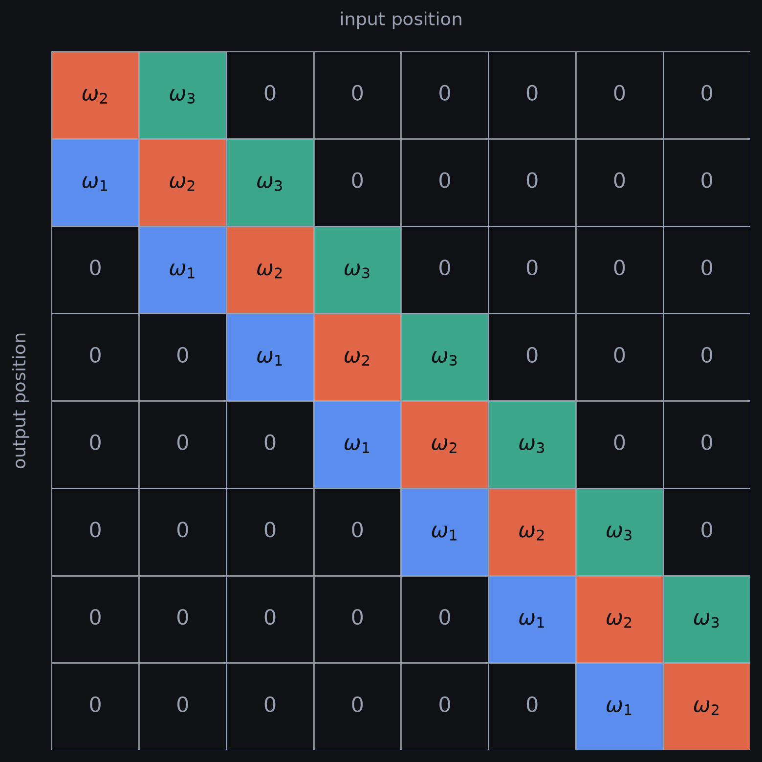
The convolution with kernel size three, zero padding and eight inputs, written as the dense matrix that computes it. Each colour is one kernel weight, repeated down its diagonal; every other entry is a structural zero.
Boundaries and spatial scale
Boundaries
- A width-3 kernel centred on \(x_1\) needs \(x_0\), which doesn’t exist
- Two choices
- invent values beyond the edge so the kernel still applies
- compute outputs only where the whole kernel fits
- Each choice changes the output size and the behaviour at the edges
Padding
- Zero padding treats every value outside the input as zero
- Other boundary assumptions
- reflection
- circular wrapping
- Padding invents values beyond the boundary: it states an assumption about what lies there.
Definition 4 Padding extends the input by \(P\) positions at each end before the kernel is applied. Zero padding fills those positions with zeros.
Valid convolution
- Keep only the positions where the whole kernel lies inside the input
- Input length \(\din\), kernel size \(K\), kernel evaluated at every position
\[ \dout = \din-K+1 \]
- No invented edge values
- The output is shorter than the input
Definition 5 A valid convolution evaluates the kernel only where every tap falls inside the input. It uses no padding.
Stride
- Evaluate the kernel at every \(S\)th position instead of every position
- \(S=1\): every position
- \(S=2\): every second position
Definition 6 The stride \(S\) is the distance, in input positions, between the windows of consecutive outputs.
Kernel size
- A wider kernel
- sees more neighbouring positions in one layer
- uses more weights
- captures larger local patterns directly
- A narrower kernel
- uses fewer parameters
- builds wider context gradually, through depth
Dilation
- Space the kernel’s taps apart: the same number of weights, a wider reach
- For a 3-tap kernel at position \(i\), with dilation \(\delta\), read “delta”
- \(\delta=1\): positions \(i-1,i,i+1\)
- \(\delta=2\): positions \(i-2,i,i+2\)
- \(\delta=3\): positions \(i-3,i,i+3\)
- Effective kernel width, read “K effective”
\[ K_{\text{eff}}=1+\delta(K-1) \]
- \(K=3\), \(\delta=2\): \(K_{\text{eff}}=5\), positions \(i-2\) to \(i+2\)
Definition 7 The dilation \(\delta\) is the distance, in input positions, between adjacent taps of the kernel. An ordinary kernel has \(\delta=1\).
Output size
- Input length \(\din\), padding \(P\) at each end, kernel size \(K\), dilation \(\delta\), stride \(S\)
\[ \dout= \left\lfloor \frac{\din+2P-K_{\text{eff}}}{S} \right\rfloor+1, \qquad K_{\text{eff}}=1+\delta(K-1) \]
- Reading it
- \(\din+2P\): the padded length
- \(\din+2P-K_{\text{eff}}\): how far the window can slide
- divide by \(S\): one output per step
- \(+1\): the window’s first position
- Valid, \(S=1\), \(\delta=1\): \(\dout=\din-K+1\), as before
- \(S=1\), \(\delta=1\), odd \(K\), \(P=(K-1)/2\): \(\dout=\din\), so the size is kept
- Seven inputs, no padding, \(K=3\), \(S=2\): \(\lfloor(7-3)/2\rfloor+1=3\)
Padding, stride and dilation compared
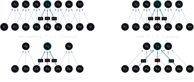
Seven inputs and a kernel of size three under four settings. Every output’s connections are drawn faintly; one output’s three are in colour, each carrying its weight. Padding adds zeros at the edges; stride spaces the outputs; dilation spaces the taps.
Channels
Channels and feature maps
- One kernel detects one kind of local pattern
- A useful representation needs many
- rising and falling edges
- horizontal and vertical structure
- different textures
- learned combinations of earlier features
- So a layer applies many kernels in parallel
Definition 8 A channel is one array of values over the spatial positions. In a hidden convolutional layer, each output channel is often called a feature map because it records one learned feature across positions.
Three kernels, three channels
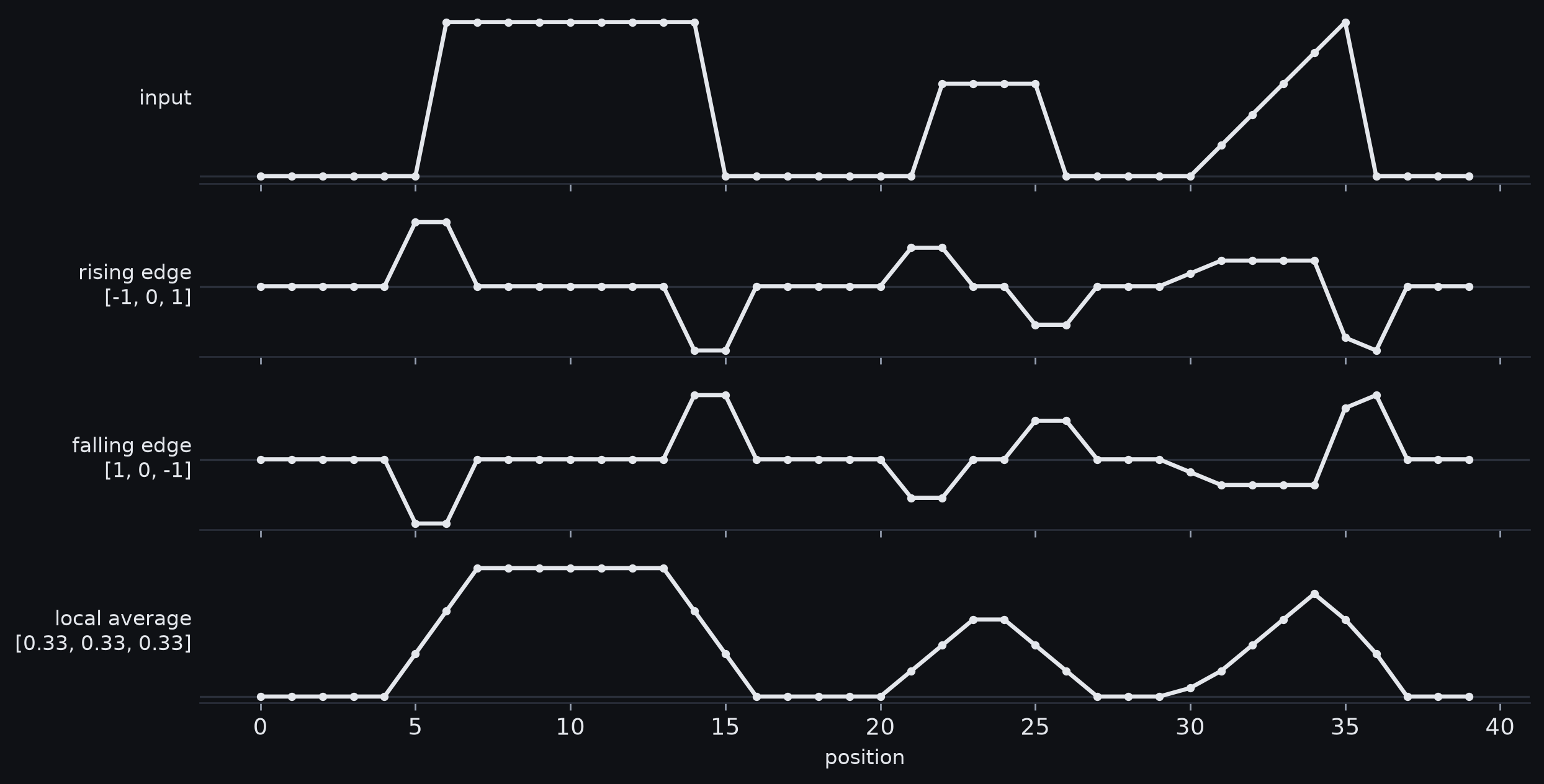
One 1D signal, top, and the three feature maps that three different kernels produce from it, on the same positions. Each row is one channel: the same signal, a different local question. The rising-edge map is positive where the signal climbs, the falling-edge map is its mirror, and the average is a smoothed copy.
Multi-channel input
- \(C_i\) input channels and \(C_o\) output channels, read “C in” and “C out”; kernel size \(3\)
- Output channel \(c\) at position \(i\) reads every input channel across the window
\[ h_{ci}=\activation{\beta_c+\sum_{c'=1}^{C_i}\sum_{j=1}^{3}\omega_{c'cj}\,x_{c',i+j-2}} \]
- Read \(\omega_{c'cj}\) as “omega c-prime c j”: the weight from input channel \(c'\) to output channel \(c\) at tap \(j\)
- Sum over every input channel \(c'\) and every tap \(j\), then add channel \(c\)’s bias
- With \(C_i=C_o=1\) this is the single-channel unit from before
- For \(C_o\) output channels and kernel size \(K\): \(C_iK\) weights and one bias per output channel
\[ \layerweights\in\reals^{C_i\times C_o\times K}, \qquad \layerbias\in\reals^{C_o}, \qquad \text{parameters}=C_o(C_iK+1) \]
- PyTorch stores the same weights as \(C_o\times C_i\times K\)
Position and channel
- A hidden representation has two kinds of axis
- Position: where in the signal the response occurred
- Channel: which learned measurement produced it
- Convolution mixes nearby positions, and combines every input channel as it does so
Receptive fields
Receptive field
- With width-3, stride-1 convolutions
- a layer-1 unit depends on 3 input positions
- a layer-2 unit on 5
- a layer-3 unit on 7
- Depth composes local operations into wider context
Definition 9 The receptive field of a hidden unit is the region of the original input that can influence it.
Receptive fields by stride
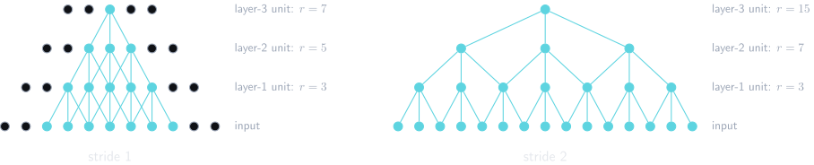
Three convolutional layers with kernel size three. The highlighted unit at the top and every unit that can influence it. Left, stride one: the receptive field grows by two per layer. Right, stride two: 3, 7, then 15 positions, because each layer’s taps sit twice as far apart as the last’s.
Receptive field at stride 1
- Stride \(1\), kernel width \(K\), after \(L\) layers
\[ r_L = 1 + L(K-1) \]
- For \(K=3\): \(r_L=1+2L\)
- With the same dilation \(\delta\) in every layer, the field spans \(r_L=1+L\delta(K-1)\) positions, with gaps: only \(1+L(K-1)\) of them feed the unit
- dilations that double layer by layer fill the gaps
Receptive field with stride
- With stride above one, neighbouring hidden units sit further apart in the input
- Track two quantities, starting at the input with \(r=1\) and \(J=1\)
- receptive-field width \(r\)
- jump \(J\): the spacing between adjacent hidden units, in input positions
- A layer with kernel \(K\), stride \(S\) and dilation \(\delta\) updates them, using the incoming \(J\)
\[ \begin{aligned} r' &= r + (K-1)\delta J\\ J' &= SJ \end{aligned} \]
- The \(K\) taps read units \(\delta J\) input positions apart, so the window reaches \((K-1)\delta J\) further
- Each stride-\(S\) layer multiplies \(J\) by \(S\), so later taps sit further apart in the input
- Three layers with \(K=3\), \(S=2\), \(\delta=1\)
| Layer | \(r\) | \(J\) |
|---|---|---|
| input | 1 | 1 |
| 1 | 3 | 2 |
| 2 | 7 | 4 |
| 3 | 15 | 8 |
- Each row’s \(r\) uses the row above’s \(J\): \(3+2\cdot2=7\), then \(7+2\cdot4=15\)
MNIST-1D
MNIST-1D
- From last Friday: a synthetic one-dimensional analogue of MNIST (Greydanus and Kobak 2020)
- The chapter’s experiment
- input: \(40\) values
- output: \(10\) class activations, then softmax
- training set: \(4{,}000\) examples
- The data include random translations of underlying templates
- so sharing weights across positions is a sensible prior to test
The convolutional model
- \(3\) convolutional hidden layers, each with
- \(15\) channels
- kernel size \(3\)
- stride \(2\)
- valid convolution
- Spatial sizes: \(40\rightarrow19\rightarrow9\rightarrow4\)
- Final hidden representation: \(4\times15=60\) values
- Then a fully connected map to \(10\) outputs
MNIST-1D results
- Parameters
- convolutional network: \(2{,}050\)
- fully connected network: \(59{,}065\)
- Both fit the training data perfectly
- Test error after training, our re-run, mean of 3 seeds
- convolutional: 14.5%
- fully connected: 40.6%
- The dense network can represent the CNN’s mapping; SGD finds a different perfect fit instead, which generalises worse
Training and test error
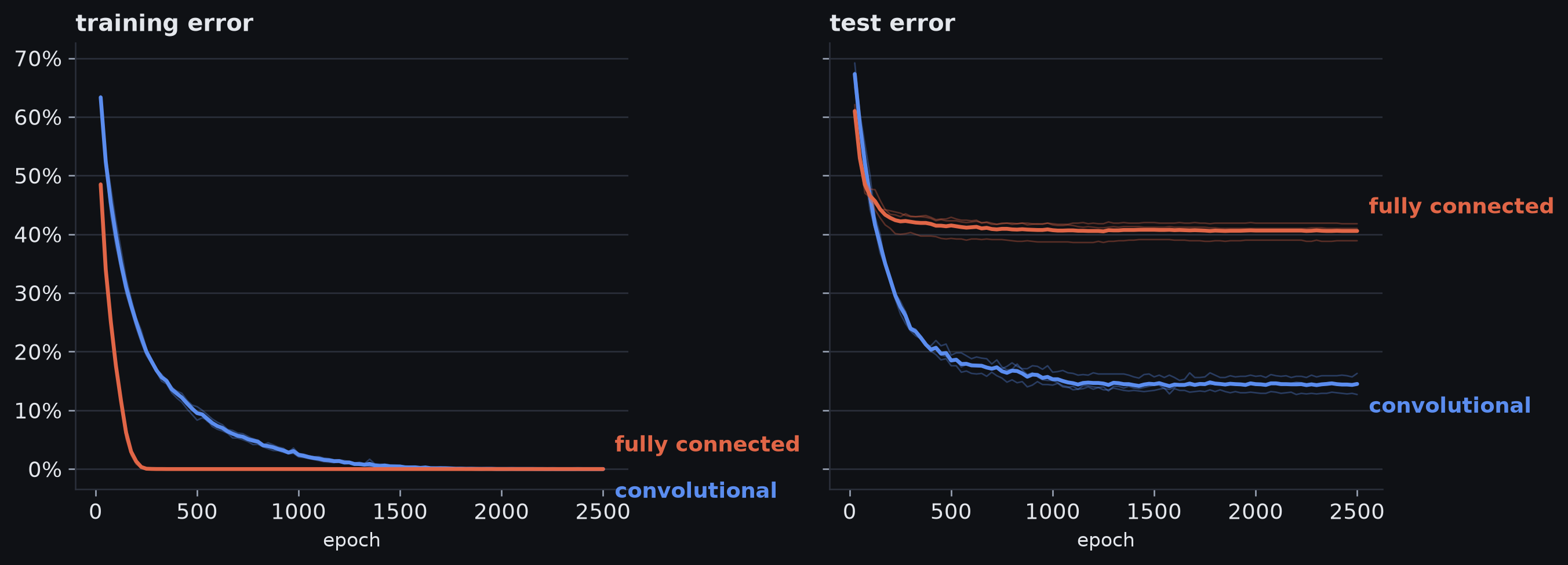
Our re-run of the chapter’s MNIST-1D comparison: SGD at learning rate 0.01, batch size 100, 100,000 steps, three seeds each. Left: both networks reach zero training error. Right: test error, where the convolutional network ends far lower.
Interpreting the result
- Tempting reading: the CNN generalises better because it has fewer parameters
- this comparison doesn’t establish that
- The result is consistent with an inductive-bias explanation
- the data contain translated versions of related patterns
- the CNN is forced to reuse detectors across position
- the dense network is free to learn unrelated behaviour at different positions
Restricted hypothesis space
- The hypothesis space is the family of functions an architecture can represent
- A dense network is free to use different weights at every position
- A convolutional network is not
- interactions are local
- weights are shared across position
- Those constraints rule out many mappings before training begins
- Prince’s explanation: a CNN searches a smaller family of mappings, all of them plausible (Prince 2023)
- alternatively, the architecture acts as a regulariser with an infinite penalty on most of the dense network’s solutions
Convolution in 2D
2D kernels
- A \(3\times3\) kernel on a single-channel image reads nine neighbouring values
- The patch at position \((i,j)\)
\[ \begin{bmatrix} x_{i-1,j-1} & x_{i-1,j} & x_{i-1,j+1}\\ x_{i,j-1} & x_{i,j} & x_{i,j+1}\\ x_{i+1,j-1} & x_{i+1,j} & x_{i+1,j+1} \end{bmatrix} \]
- The same \(3\times3\) weights are reused across the whole image
2D convolution
- With kernel weights \(\omega_{mn}\)
\[ h_{ij}= \activation{ \beta+ \sum_{m=1}^{3}\sum_{n=1}^{3} \omega_{mn}x_{i+m-2,j+n-2} } \]
- take the \(3\times3\) patch around \((i,j)\)
- multiply it by the kernel, elementwise
- sum
- add the bias
- apply the activation
Three kernels on a digit
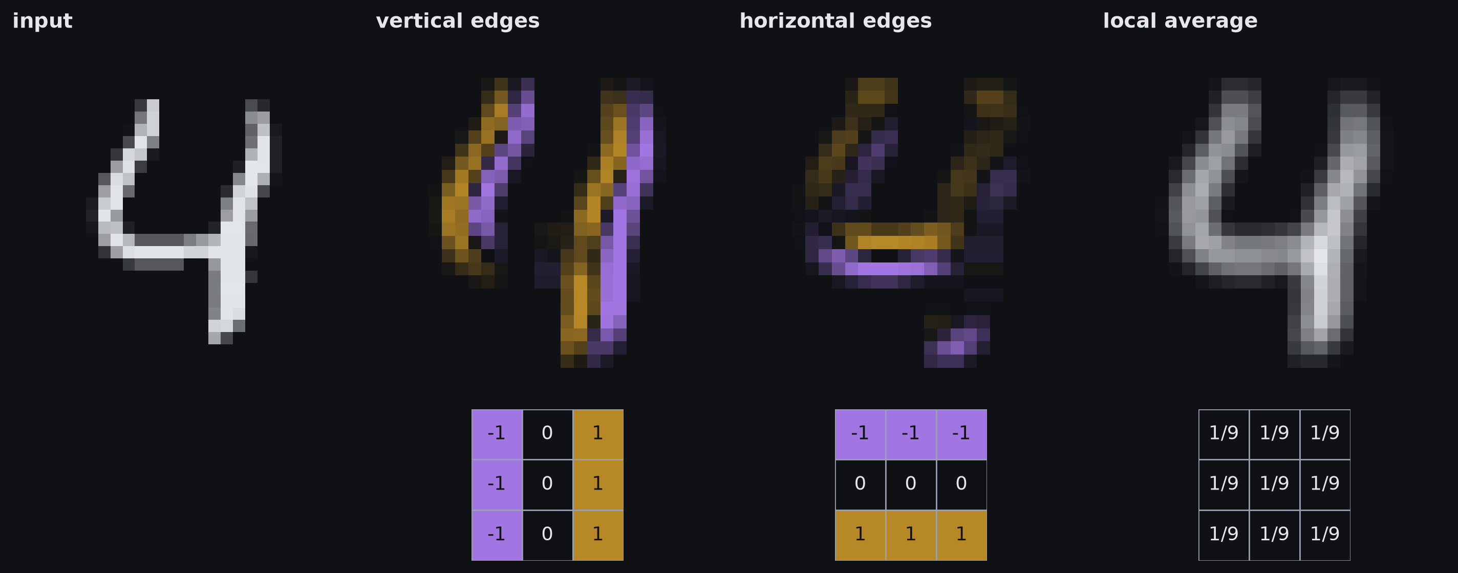
A real MNIST digit, left, and what three 3 x 3 kernels compute from it, each kernel’s weights drawn under its output. The edge kernels respond with opposite signs on the two sides of a stroke, in the same colours as the negative and positive weights that produce them. The averaging kernel blurs. MNIST, LeCun and Cortes, CC BY-SA 3.0.
Colour channels
- An RGB image has three channels, each an \(H\times W\) array
- A \(3\times3\) kernel for one output channel spans all three
- \(3\times3\times3=27\) weights
- A 2D kernel covers every input channel across one spatial patch.
2D parameter count
- Kernel size \(K\times K\), \(C_i\) input channels, \(C_o\) output channels
- Weights and biases
\[ \layerweights\in\reals^{C_i\times C_o\times K\times K}, \qquad \layerbias\in\reals^{C_o} \]
- Parameter count
\[ C_o(C_iK^2+1) \]
Dense and convolutional scaling
- For a \(224\times224\times3\) image
- Dense: input values times outputs, so the image size enters twice
- Convolutional: \(C_o(C_iK^2+1)\), with no image size in it
- For fixed kernel sizes and channel counts, a bigger image means more kernel evaluations but the same number of convolutional parameters
- Same image
- Convolution: 64 kernels of \(3\times3\) need \(64(3\cdot3\cdot3+1)=1{,}792\) parameters
- Dense: one layer from the image to an output of its own size needs about \(2.27\times10^{10}\)
Downsampling
Cost of resolution
- Keeping full \(H\times W\) resolution through every layer increases
- memory use
- computation
- It also means receptive fields grow relatively slowly in input coordinates
- CNNs therefore often shrink spatial size as depth grows
- fewer positions to compute
- wider context per remaining position
- often more channels
- Resolution: downsampling reduces the number of positions at which information is represented
- Channels: extra channels can represent more kinds of feature at each remaining position
- Increasing channels as resolution falls is a common design choice, not a mathematical law
Downsampling methods
| Method | Operation on each local region |
|---|---|
| Stride-2 convolution | a learned weighted combination, evaluated at every second position |
| Max pooling | keep the largest value |
| Mean pooling | average the values |
Definition 10 Pooling with block size \(k\) replaces each non-overlapping \(k\times k\) block of a channel by one number, its maximum or its mean. Each channel is pooled separately, so its \(H\times W\) array becomes \(H/k\times W/k\), when \(k\) divides both, and the channel count is unchanged.
- A strided convolution mixes channels, like every convolution in this lecture
Max pooling
- Max pooling keeps the strongest response in each block and discards its exact position
\[ \max \begin{bmatrix} 0.2 & 1.7\\ 0.9 & 0.4 \end{bmatrix} =1.7 \]
- A small shift can move the peak within its block and leave the pooled value unchanged
- Max pooling ignores a shift whenever each block’s largest value stays inside that block, and stays the largest.
Mean pooling
- Mean pooling keeps the average response in each block and discards the internal arrangement
\[ \operatorname{mean} \begin{bmatrix} 0.2 & 1.7\\ 0.9 & 0.4 \end{bmatrix} =0.8 \]
- Compared with max pooling
- max asks “was there a strong response here?”
- mean asks “how much response was there, on average?”
- Each keeps one number per block
- max: the largest value, not how many values were large
- mean: the average, not where it came from or how high the peak was
Pooling under a shift
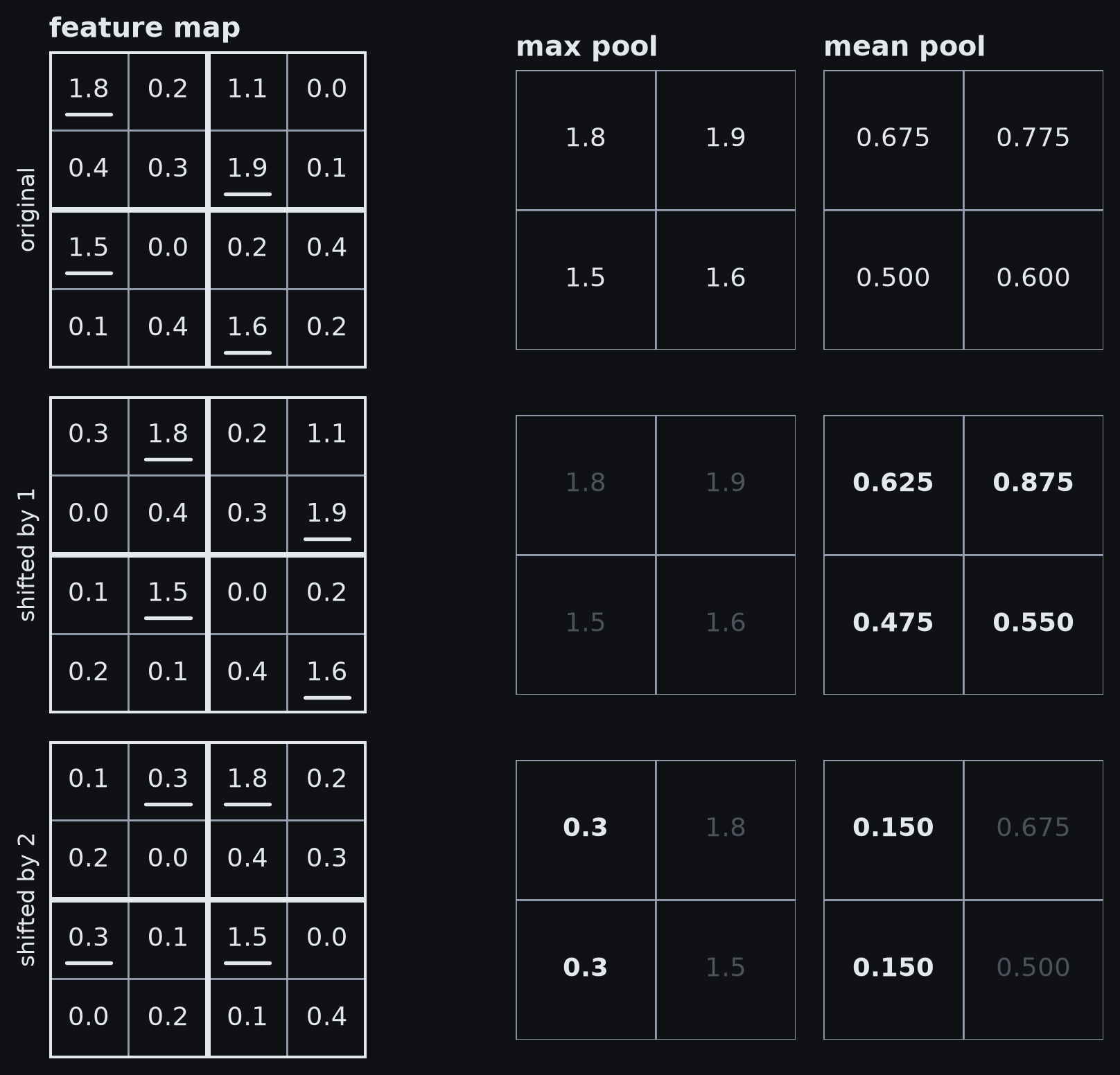
A 4 x 4 feature map, then the same map shifted right by one and by two, each pooled over the 2 x 2 blocks outlined. Each block’s largest value is underlined. In the shifted rows, a faded pooled value is one the original already had: in the same cell after a shift of one, one cell to the right after a shift of two. Bold is new. Shifted by one, every peak stays in its block, so max pooling is unchanged while mean pooling changes. Shifted by two, the pooling step, both pooled maps move one cell right; only the column filled from the edge is new.
Upsampling
Dense prediction
- Classification can end in one class vector
- Segmentation needs an output at every pixel
- So a common shape is
\[ \text{high resolution} \rightarrow \text{compressed representation} \rightarrow \text{high resolution} \]
- The first half gathers context; the second restores spatial scale
Fixed upsampling
- Upsampling without learned weights
- nearest-neighbour duplication
- bilinear interpolation
- max unpooling: record where each maximum came from in the encoder, and put values back there
- None of these learns new detail; max unpooling only reuses positions saved from the encoder
Transposed convolution
- Write a stride-2 convolution as a matrix product: \(\vect{z}=\layerweights\vect{x}\)
- A transposed convolution applies a matrix with the sparsity and sharing pattern of \(\layerweights\transpose\)
- it maps a coarse spatial representation to a finer spatial grid
- its weights are its own, learned like any other layer’s, not copied from the encoder
- it’s named for the transposed matrix; it is not the inverse
A strided convolution and its transpose
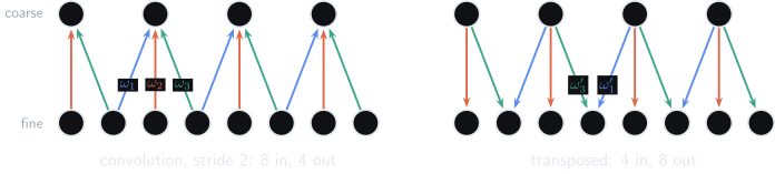
Left: a stride-2 convolution with kernel size three and zero padding, from eight fine positions to four coarse ones. Right: its transpose, from four back to eight. The same eleven connections and the same sharing pattern, with the arrows reversed; the primed weights are the transposed layer’s own. A fine unit now receives two contributions or one, depending on where it sits.
Transpose and inverse
- Transpose: swap the map’s input and output roles, in the matrix sense
- Inverse: recover the exact original input
- This stride-2 convolution maps 8 values to 4, so no inverse exists
- A transposed convolution learns a map from coarse to fine; it can’t restore what was lost
Channel mixing
Channel mixing with \(1\times1\) convolution
- At stride \(1\), a \(1\times1\) convolution does no spatial processing: it mixes features at each location
- If a position has \(C_i\) learned measurements, it can learn \(C_o\) new combinations of them
- At position \((i,j)\) the hidden vector is \(\hidden_{ij}\in\reals^{C_i}\); the subscript names the position
- A \(1\times1\) convolution computes
\[ \vect{z}_{ij}=\layerbias+\layerweights\transpose\hidden_{ij}, \qquad \layerweights\in\reals^{C_i\times C_o} \]
- \(\layerweights\) is the \(1\times1\) kernel, \(C_i\times C_o\) as before; the transpose makes it act on \(\hidden_{ij}\)
- a matrix transpose of the kernel, not a transposed convolution
- The same channel-mixing map is applied at every \((i,j)\)
- It’s a fully connected layer applied to the channel vector at each pixel
Uses of \(1\times1\) convolution
- It can
- reduce the channel count
- expand the channel count
- recombine learned features
- match channel counts before branches merge
- It does not mix neighbouring positions
Classification, detection and segmentation
Output shapes by task
| Task | Output | Meaning |
|---|---|---|
| Classification | one score per class | one class distribution for the image |
| Object detection | classes and boxes at many locations | what is where |
| Semantic segmentation | \(H\times W\) scores per class | one class distribution per pixel |
- For an RGB image, the input is three \(H\times W\) channels; what changes between tasks is the required output structure
Classification networks
- keep local spatial structure through the convolutional layers
- downsample gradually while adding channels
- integrate information across the whole image: fully connected layers in AlexNet and VGG, global pooling in many later networks
- map to class activations
- apply softmax for class probabilities
- For ordinary image classification, the prediction should not depend on where the object appears
- So position can be collapsed near the end
AlexNet: the early CNN pattern
- Input: \(224\times224\) colour image (Prince 2023)
- Five convolutional hidden layers followed by three fully connected stages
- Uses ReLU activations and max pooling
- About \(60\) million parameters
- The architectural pattern is the important part
- convolution preserves and transforms spatial structure
- pooling progressively reduces spatial resolution
- fully connected stages produce the final classification
- Training also used data augmentation, SGD with momentum, dropout and L2 weight decay
VGG: greater depth
- Repeated convolution and max pooling
- Spatial size falls as channel count grows
- Fully connected layers produce the final classification
- The 19-layer variant had about \(144\) million parameters (Prince 2023)
- For several years, deeper networks improved ImageNet results
- Past a point, simply adding depth made networks difficult to train without architectural changes
Object detection
- Detection predicts several objects and where each one is
- In early YOLO, a \(7\times7\) grid is placed over the image (Prince 2023); each cell predicts
- class information
- a fixed number of boxes, two in the original, each with
- centre \((x,y)\)
- width and height
- confidence
- The output keeps enough spatial layout to locate objects
Duplicate detections
- A detector can produce several boxes for one object
- Non-maximum suppression (NMS) removes overlapping lower-confidence boxes after prediction
- Keep two stages distinct
- network output: candidate boxes
- inference pipeline: candidate boxes plus post-processing such as NMS
Semantic segmentation
- For a \(224\times224\) image and \(21\) classes, a segmentation network can output \(224\times224\times21\) values (Prince 2023)
- Softmax at each position turns \(21\) activations into class probabilities
- The output is on the input’s pixel grid; the target mask moves with the object, which is the equivariance the task asks for
Encoder–decoder shapes
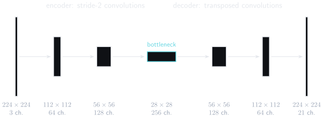
A schematic segmentation network’s tensor shapes, not the chapter’s network. Height is side length; width grows with channel count, floored so the thinnest stay visible. Three stride-2 convolutions halve the image three times while channels grow; three transposed convolutions restore it, ending in one score per class at every pixel.
Encoder and decoder
- Encoder
- downsamples step by step
- increases receptive field
- represents progressively less local features across more channels
- Decoder
- upsamples
- returns to full spatial resolution
- turns hidden channels into per-pixel predictions
- The network has to see a wide region of the image to label each pixel locally
Assumptions and limits
Hypothesis space
- Compared with a dense layer, convolution assumes
- locality matters
- the same local computation is useful at every position
- a shifted input should give a shifted representation
- These constraints remove many possible mappings from input to output
- If a good mapping survives the restriction, training searches a smaller family to find it
- MNIST-1D fits this picture; it illustrates the idea rather than proving it
When weight sharing fits
- Useful when
- a pattern means roughly the same thing wherever it appears
- local structure repeats across space
- Limiting when
- absolute position matters
- the important relationships are long-range
- translation isn’t the right symmetry
- An inductive bias helps only when its assumptions match the problem.
Downsampling trade-offs
- Gains
- less computation
- larger receptive fields
- reduced sensitivity to small shifts; with max pooling, exact invariance to shifts that keep each block’s maximum inside it and still the largest
- Losses
- precise location
- fine detail
- distinctions smaller than the pooling or stride scale
- So a network that downsamples needs a way back to full resolution for dense prediction: a decoder path, or the skip connections of later architectures
Other symmetries
- Of the geometric transformations, standard convolution is equivariant only to translation
- It is neither invariant nor equivariant by construction to
- rotation
- scale
- reflection
- perspective
- elastic deformation
- Data augmentation or specialised architectures handle these separately
Revision
Core vocabulary
- Inductive bias: a learning system’s tendency to favour some solutions over others
- Invariance: the input moves, the output stays the same
- Equivariance: the input moves, the output moves the same way
- Kernel, or filter: the shared local weights
- Cross-correlation: the unflipped sum that deep-learning libraries call convolution
- Kernel size: the number of taps \(K\); with dilation, the extent is \(K_{\text{eff}}\)
- Stride: the spacing between kernel evaluations
- Padding: the rule for values beyond the boundary
- Dilation: the spacing between kernel taps
- Channel: one array of values over positions; in a hidden layer, a feature map
- Pooling: one number per block, per channel
- Receptive field: the region of the input that can affect a hidden unit
- Transposed convolution: a learned coarse-to-fine map with \(\layerweights\transpose\)’s pattern, not an inverse
Kernel size, stride, dilation and channels
| Quantity | Changes |
|---|---|
| Kernel size | taps: local extent, and parameters |
| Stride | output sampling density and spatial size |
| Dilation | spatial extent, without adding taps |
| Number of channels | number of learned response types |
Output size and receptive field
- Output size
\[ \dout=\left\lfloor\frac{\din+2P-K_{\text{eff}}}{S}\right\rfloor+1, \qquad K_{\text{eff}}=1+\delta(K-1) \]
- Receptive field at stride \(1\): \(r_L=1+L(K-1)\)
- With stride: \(r'=r+(K-1)\delta J\) and \(J'=SJ\), from \(r=J=1\) at the input
Padding and valid convolution
- Padding
- evaluates near boundaries
- can keep the spatial size
- assumes something beyond the edge
- Valid convolution
- invents no boundary values
- computes only fully supported outputs
- shrinks the spatial size
Channel mixing
- A \(1\times1\) convolution maps \(\reals^{C_i}\rightarrow\reals^{C_o}\) at each position
- no neighbouring pixels are mixed
- the same channel map is reused everywhere
- the spatial size can stay unchanged
Source and revision locators
- Simon J. D. Prince, Understanding Deep Learning, Chapter 10: “Convolutional networks” (Prince 2023)
- Sections: 10.1 invariance and equivariance; 10.2 1D convolution, padding, stride, kernel size, dilation, channels, receptive fields and MNIST-1D; 10.3 2D convolution; 10.4 downsampling, upsampling and \(1\times1\) convolution; 10.5 classification, detection and segmentation
- Equations: 10.1–10.6
- Notebooks: 10.1–10.5
- Figures worth revisiting: 10.1 invariance and equivariance; 10.2–10.5 convolution mechanics and channels; 10.6 receptive fields; 10.7–10.8 MNIST-1D; 10.9–10.14 2D convolution, down- and upsampling, transposed and \(1\times1\) convolution; 10.16–10.19 AlexNet, VGG, YOLO and segmentation
- Problems: 10.1–10.19; 10.1, the equivariance derivation, is worked in lecture