an over-parameterised model can interpolate every training example
many parameter settings then reach the same, or nearly the same, training loss
those settings can behave very differently between the observed examples
Training loss says which solutions fit the observed data
It needn’t say which fitted solution behaves sensibly elsewhere
Regularisation as solution selection
Several fitted models explain the training data equally well
They behave differently between the observations
Something other than training loss has to choose
Definition 1Regularisation is any mechanism that biases learning toward a subset of the fitting solutions, to improve generalisation.
Typical preferences: smoother functions, or less sensitivity to perturbation
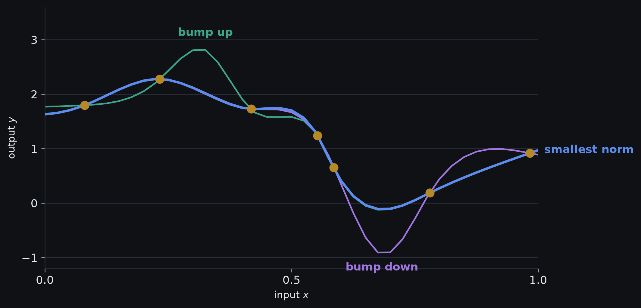
Interpolants of the same points
Three functions that pass exactly through the same seven training points, so all three have zero training loss. Blue is the smallest-norm fit; the other two add a bump between two observations, where no training point can see it. Training loss cannot choose between them.
Strict and broad senses of regularisation
Strict sense: an explicit term added to the loss
the objective itself changes
Broad sense: any strategy intended to improve generalisation
the objective may be unchanged
This session: explicit regularisation formally first, then the broad sense
An optimiser needs one scalar objective to compare candidate parameter settings
The data loss already gives one score: how badly the model fits the observations
\(g[\params]\) gives a second score: how strongly a parameter setting violates the preference we want to impose
\(\lambda\) sets the exchange rate between those two scores
The penalty is therefore not another measurement from the data
It is a modelling choice about which fitting solutions we would rather select when data fit alone does not decide
Regularisation and the optimum
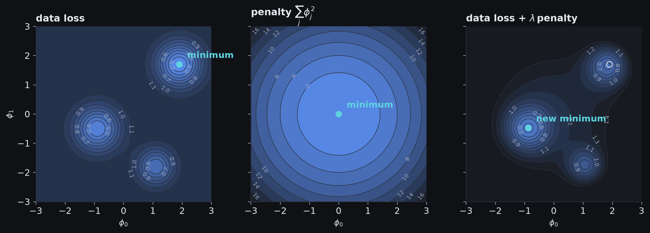
The regularised objective is a different surface from the data-fitting loss.
Loss, penalty and their sum
Left: a data-fitting loss over two parameters with three basins; the lowest is marked. Centre: an L2 penalty, smallest at the origin. Right: their sum. The penalty raises the far basin more than the near one, so the global minimum of the sum moves to a different basin.
Parameter magnitude gives a simple generic preference
The interpolating models from the opening all fit the observed points
They can nevertheless require very different parameter values
A simple generic preference is: when fit is comparable, favour parameters closer to zero
In one dimension, distance from zero is just \(|\phi|\)
With many parameters, we need one number that measures their combined magnitude
Small parameter magnitude is a proxy, not a theorem about simple functions
Neural networks can be reparameterised, so the same function can sometimes be represented with different weight scales
L2 is Euclidean length in parameter space
Remember how Pythagoras combines movement along perpendicular axes?
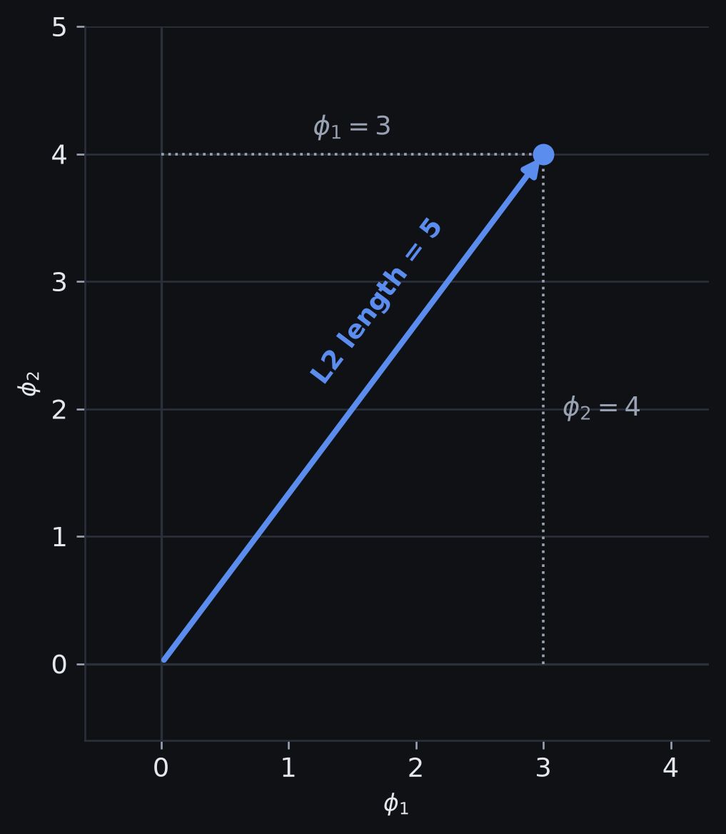
Example: \(\params=[3,4]^{\top}\) has \(\norm{\params}_2=5\)
Every coordinate contributes to the overall length
Moving farther from zero in any direction increases the norm
Only the distance matters: parameter vectors at the same radius receive the same L2 magnitude
L2 is distance from the origin
In two parameter dimensions, the L2 norm is ordinary Euclidean distance from the origin. The vector [3,4] has length 5 by Pythagoras. An L2 penalty therefore charges according to how far the whole parameter vector lies from zero, not according to any one coordinate alone.
Why prefer smaller weights?
A neural-network layer forms weighted sums of its inputs or activations
A large weight acts like a large gain: a change upstream can produce a larger change downstream
Large gains across several layers can make the fitted function highly sensitive to small changes
L2 gives a soft preference against relying on very large gains
it does not forbid them when the data strongly support them
Intuition: smaller weights can make the network less eager to produce sharp changes from small upstream differences
Caveat: parameter magnitude is only a proxy for function behaviour
neural networks can sometimes represent the same function with different weight scales
Squared L2 is convenient for optimisation
Regularisation normally uses
\[
\norm{\params}_2^2
=
\sum_{j=1}^{P}\phi_j^2
\]
rather than the square root itself
squaring preserves the ordering: the vector with smaller L2 norm also has smaller squared L2 norm
the derivative is simple: \(\nabla_{\params}\norm{\params}_2^2=2\params\)
large coordinates become disproportionately expensive
the penalty is smooth everywhere
So L2 regularisation says: fit the data, but pay an increasing cost for moving far from the origin in parameter space
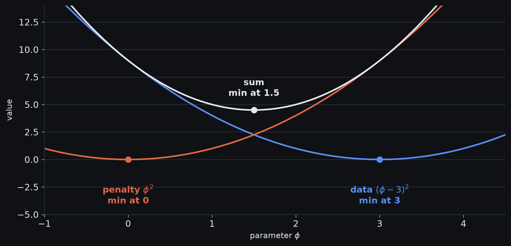
Squared L2 in one parameter
Data term alone, minimised at \(\phi=3\):
\[
\loss_{\text{data}}(\phi)=(\phi-3)^2.
\]
Add an L2 penalty with \(\lambda=1\):
\[
\loss_{\text{reg}}(\phi)=(\phi-3)^2+\phi^2.
\]
Data term: minimised at \(3\)
Penalty: minimised at \(0\)
Sum: a compromise between them
The one-parameter example
The data-fitting loss is minimised at φ = 3, the L2 penalty at φ = 0, and their sum at φ = 1.5: the regularised optimum gives up some data fit for a smaller parameter.
The regularised optimum
Commit first: which \(\phi\) minimises \((\phi-3)^2+\phi^2\)?
In neural networks, L2 is usually applied to the weights, not the biases
So \(\lambda\sum_k\norm{\layerweights_k}_F^2\) doesn’t penalise every scalar in \(\params\)
Probabilistic reading: no L2 prior penalty is imposed on the biases in this formulation
In code: biases go in their own optimiser parameter group, with zero decay
Small weights in the toy model
In the simplified piecewise-linear network:
each layer forms weighted sums
large weights allow larger changes in downstream pre-activations
penalising weight magnitude discourages those changes
Limit: with every weight zero, the output becomes a constant: the final bias
Scope: explains this toy model’s smoothing
not a theorem that smaller weights make every network smoother
L2 strength and the fitted function
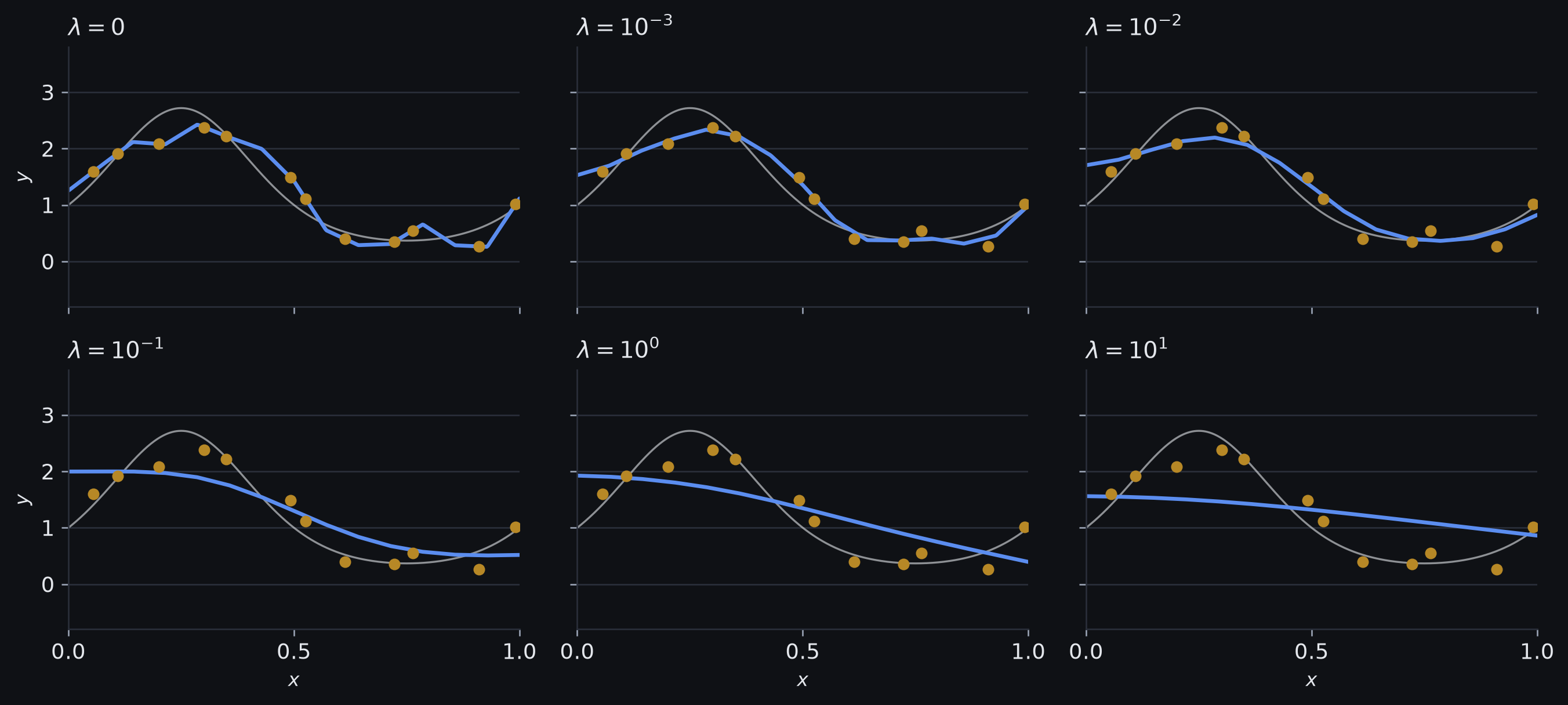
The same twelve training points and the same fourteen-joint model, fitted with increasing L2 strength λ. With no penalty the fit chases the noise; moderate λ removes the sample-specific bends; large λ removes the underlying shape as well. The thin grey curve is the true mean.
Regularisation strength, bias and variance
As \(\lambda\) increases:
training fit generally worsens
sensitivity to sample-specific variation can fall
the fitted function becomes more constrained
too much constraint underfits
One mechanism can reduce variance while increasing bias.
Choosing \(\lambda\): a hyperparameter, set on validation evidence
PyTorch SGD’s weight_decay=wd adds \(wd\,\params\) to the gradient
For the same data-loss reduction, the coefficients correspond as:
\[
wd=2\lambda.
\]
Plain SGD, no momentum: the direct shrinkage coefficient at step \(t\) is
\[
\lambda'_t=\alpha_t\,wd
\]
Momentum or adaptive optimisers: derive the effect from the actual update rule
Sum to mean: rescale the L2 coefficient first
Adaptive scaling
Adaptive optimisers rescale each gradient coordinate using its history
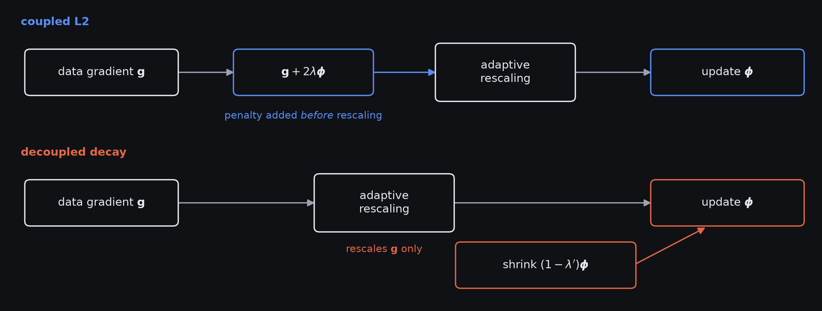
Coupled L2: \(2\lambda\params\) joins the gradient before the rescaling
so it’s transformed along with the data gradient
Direct shrinkage: skips that transformation
The motivation for decoupled weight decay in AdamW
Coupled L2 and decoupled decay
Two update rules for an adaptive optimiser. Top, coupled L2: the penalty’s gradient 2λφ joins the data gradient g before the adaptive rescaling, so each coordinate’s penalty is rescaled too. Bottom, decoupled weight decay (AdamW): only g is rescaled, and the shrinkage is applied to φ on a separate branch. Under plain SGD there is no rescaling and the two coincide.
Coupled and decoupled decay in PyTorch
# SGD adds weight_decay * parameter to the gradientsgd = torch.optim.SGD( weight_params, lr=lr, weight_decay=wd,)# Decoupled weight decay for Adam-style optimisationadamw = torch.optim.AdamW( weight_params, lr=lr, weight_decay=wd,)
Give biases a separate parameter group with zero decay
Different norms encode different preferences
The penalty defines what counts as an expensive parameter vector
L2: \(\sum_j\phi_j^2\)
increasingly expensive large coordinates
smooth shrinkage toward zero
L1: \(\sum_j|\phi_j|\)
cost grows linearly with magnitude
favours sparse solutions; suitable optimisation can set some coordinates exactly to zero
L0-style: number of non-zero parameters
ignores magnitude and asks only how many parameters are active
Elastic net: combines L1 and L2
Choosing a norm means choosing a geometry of preference: different penalties favour different kinds of solutions
Sparsity
A hidden unit whose incoming weights are all zero contributes nothing
it can potentially be removed
Links regularisation to:
model compression
pruning
faster inference
Cost: the L0 count is discontinuous at zero
gradient-based optimisation can’t differentiate it the way it does L2
practical methods use relaxations or specialised procedures
Limits of explicit regularisation
Evidence on how much ordinary L2 itself explains generalisation is mixed
Individual weight magnitude is only an indirect proxy for function smoothness
Other norms and constraints can target more specific properties
Limit: a controlled modelling bias, not a universal explanation of why deep networks generalise
Implicit regularisation
Optimisation as solution selection
Setting: several parameter vectors reach the same training minimum
The objective has no explicit \(g[\params]\) term
The training algorithm can still reach some of those minima more readily than others
Definition 4Implicit regularisation is a systematic preference among equally good minima that comes from the training algorithm rather than from any term in the loss.
Consequence: the optimiser is part of the learning system’s inductive bias
Gradient flow isolates finite-step effects
We want to isolate an effect that is easy to miss:
the optimiser can bias the solution even when we never write a regularisation term
continuous gradient flow is the idealised limit of infinitesimally small steps
it gives us a reference path determined by the local gradient at every instant
Notation: from here \(t\) counts steps, not continuous time
\(\alpha\) plays the role of the time elapsed per step
The gradient is measured at \(\params_t\), then held fixed for the whole step
So the discrete path need not follow the continuous one
Gradient flow vs gradient descent
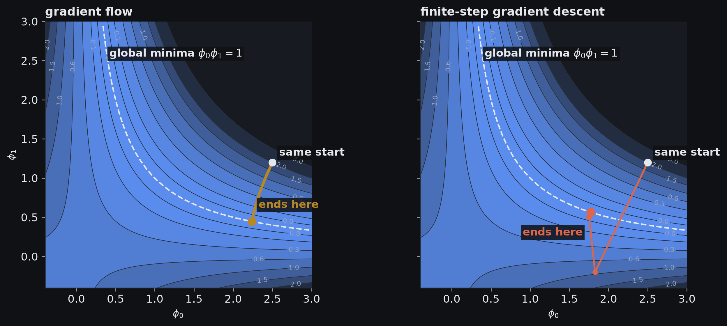
The same loss surface and the same starting point, shown separately so the trajectories are easy to compare. Left: continuous gradient flow follows a smooth curved path to one point on the valley of global minima. Right: finite-step gradient descent follows straight chords based on the gradient at the start of each step and reaches a different point on the same zero-loss valley, where the valley is wider.
The modified loss for gradient descent
Question: how far does discrete descent deviate from the continuous flow?
Reframe: which slightly modified loss would make the continuous flow track the discrete path?
Its square is large where the surface is steep in parameter space
The factor \(\alpha/4\) makes the effect stronger for larger steps
So in the modified-loss view, discrete descent is repelled from regions of large gradient magnitude
Minima under the modified loss
At an exact differentiable minimum, \(\nabla_{\params}\loss=\vect{0}\)
So the added gradient-norm term is zero there too
Every original differentiable minimum therefore remains unpenalised by this added term
The route: \(\norm{\nabla_{\params}\loss}^2\) is large on steep walls
the modified flow is pushed towards gently curved regions before it arrives
this is why finite steps can favour wider minima
What changes is the route, and so which member of a family of minima is reached.
Limits of the modified-loss approximation
The modified-loss approximation comes from a truncated backward-error expansion
only the leading-order term in \(\alpha\) is kept
Read it as: an approximate description of finite-step dynamics
Not: an exact identity for arbitrary learning rates and arbitrary training trajectories
Learning rate and implicit regularisation
In this analysis a larger \(\alpha\) does two things:
makes each step longer
strengthens the implicit gradient-norm penalty
Learning rate and test error
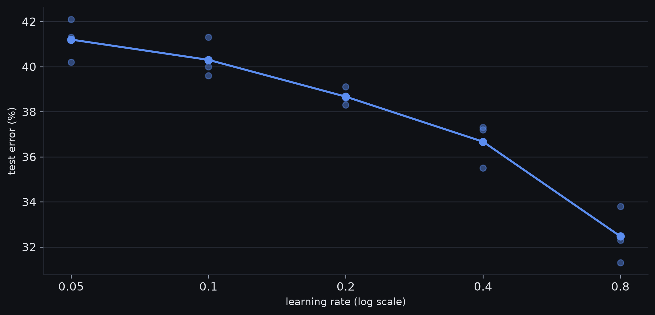
Our rerun of the chapter’s experiment: MNIST-1D, a network with two hidden layers of 100 units, SGD with batches of 100. Each run takes 6000/LR steps, so every run has the same opportunity to travel; every run fits the training set exactly. Dots are single runs from three seeds, the line their mean. Larger learning rates reach lower test error.
Reading the learning-rate result
Our rerun: the chapter’s MNIST-1D experiment, with every run given matched travel
Larger learning rates give lower test error
41% at the smallest rate, 32% at the largest
The chapter reports the same trend
Confound: these runs are minibatch SGD
so this experiment cannot isolate the full-batch finite-step mechanism from minibatch-SGD effects
What it doesn’t show:
that the largest stable learning rate is always best
that learning rate can be raised without regard to optimisation
that the gradient-norm approximation fully explains the observation
Learning rate can change which solution training reaches, as well as how fast parameters move.
Minibatch gradients
Convention: from here \(\loss\) is the mean over examples
earlier in this lecture the data-fitting objective used a sum
Batch \(b\) has its own mean loss \(\loss_b\) over its examples \(\mathcal{B}_b\)
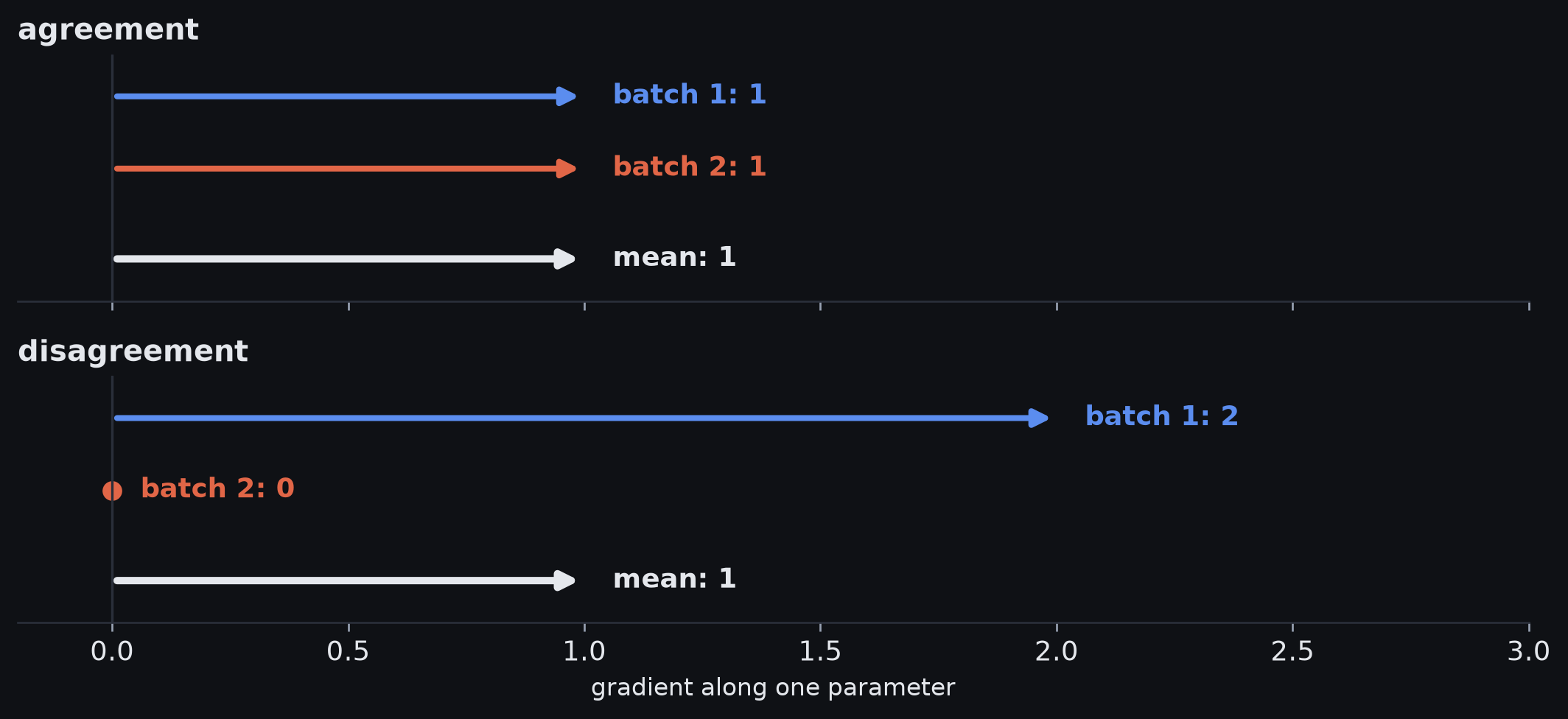
Two pairs of minibatch gradients along one parameter. Top: both batches say 1, so they agree exactly. Bottom: one says 2 and the other 0. Both pairs average to the same full gradient, 1 (white), so the mean alone cannot tell the two cases apart.
Gradient variance measures batch disagreement
The full-data gradient keeps only the average direction
That average can hide whether minibatches:
all agree closely
disagree strongly and merely cancel in the mean
Variance answers the missing question:
how far do the individual batch gradients spread around their mean?
A small variance means the batches tell a similar local story; a large variance means different subsets of the data are pulling the parameters differently
Batch-gradient variance
Batch-gradient variance: the mean squared distance of the batch gradients from their mean
Commit first: which case has the larger variance? Compute both.
Interpretation: this is the leading-order modified objective for the average SGD trajectory
The last term is absent from full-batch gradient descent
It is \(\alpha/4\) times the batch-gradient variance
Case A: \(\alpha/4\) times \(0\)
Case B: \(\alpha/4\) times \(1\)
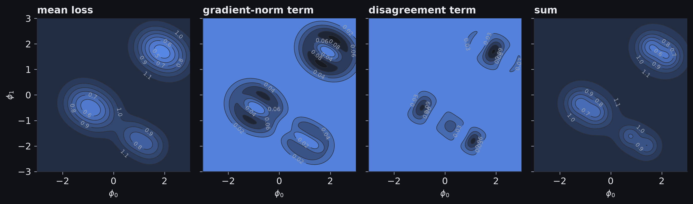
Unlike the gradient-norm term, the disagreement term need not vanish at a minimum of \(\loss\), so it can move the minimum itself.
The modified SGD surface
The pieces of the modified SGD objective, over the same two parameters, for two minibatches whose losses are the same three basins shifted slightly apart. The mean loss; the gradient-norm term (α/4)‖∇L‖²; the disagreement term, largest on the basin floors where the curvature is highest and the two shifted batches pull furthest apart; and their sum. Unlike the gradient-norm term, the disagreement term is not zero at a minimum, so the minimum of the sum moves.
Batch size and gradient disagreement
Smaller batches average over fewer examples
so individual batch gradients can vary more
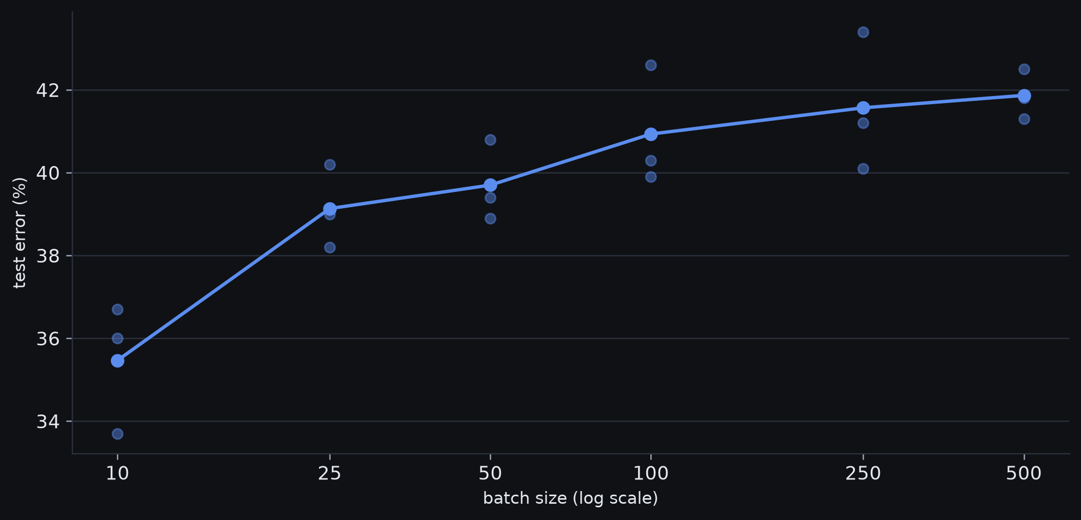
Our rerun: MNIST-1D again, each run stopped at the epoch it first fits the training set
Smaller batches reach lower test error
35% at batch size 10, 42% at 500
The chapter reports the same trend
Batch size and test error
Our rerun of the chapter’s experiment: the same network and data, SGD at learning rate 0.05, with each run stopped at the first epoch where it fits the training set exactly, so every run is compared at the point of memorisation. Dots are single runs from three seeds, the line their mean. The smallest batch reaches the lowest test error; from 25 upwards, the steps between means are smaller than the spread between seeds.
Reading the batch-size result
Implicit regularisation is one possible explanation
Batch size also changes:
gradient noise
number of updates per epoch
computational efficiency
optimisation stability
Status: “smaller batches generalise better” is an empirical tendency under some conditions, not a law
Early stopping
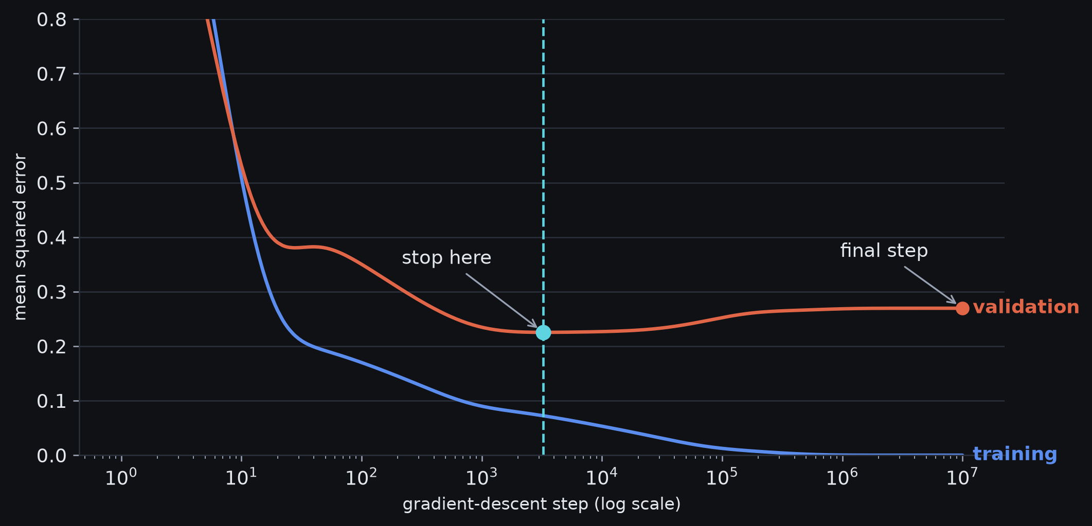
Stopping on validation loss
Training loss often keeps falling after validation performance has stopped improving
A flexible model can learn broad structure first, then sample-specific detail
Definition 5Early stopping ends optimisation before full convergence and keeps the parameters from the checkpoint with the best validation performance.
Training and validation loss
Full-batch gradient descent on the fixed-joint model from last Friday, forty joints and fourteen training points, started at zero. Training loss keeps falling towards zero; validation loss, on fresh points from the same process, reaches its minimum and then rises. Early stopping keeps the checkpoint at that minimum.
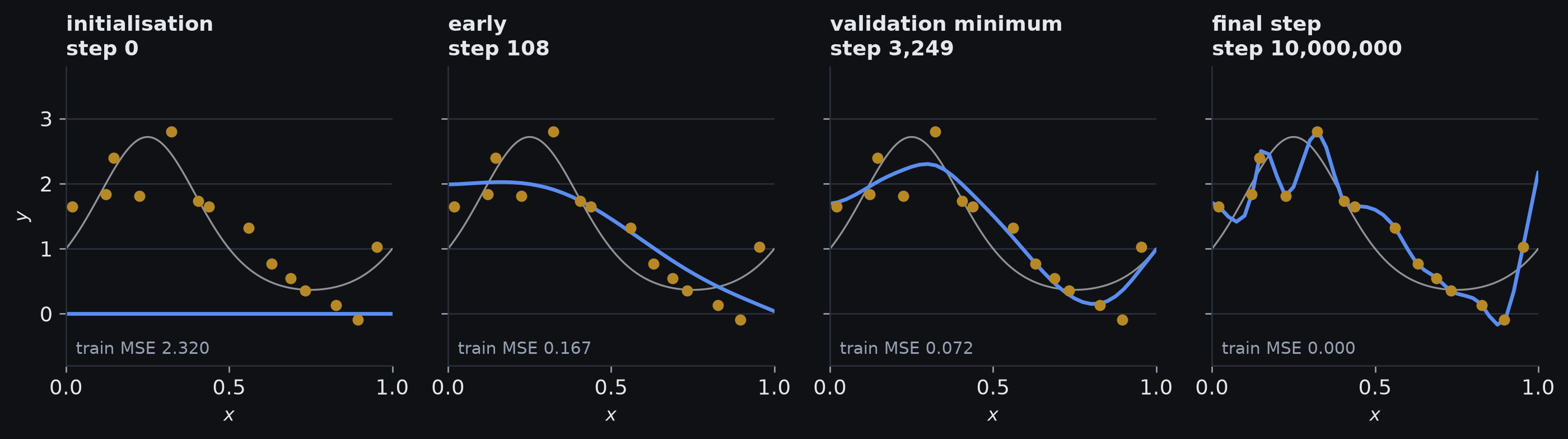
The fit during training
The same run at four moments: at initialisation, early, at the validation minimum, and at the final step. The coarse shape of the true mean (thin grey) arrives first; the late steps bend the fit through individual noisy points while training loss keeps falling.
The early-stopping hyperparameter
Hyperparameter: the effective stopping time
Chosen from a single training run:
evaluate validation performance periodically
store checkpoints
keep the checkpoint with the best validation performance
The test set stays untouched until model selection is complete
Early stopping and L2
Two intuitions:
parameters start small and have less time to grow
stopping early limits the effective complexity optimisation explores
Under a quadratic approximation with zero initialisation: early stopping is approximately equivalent to L2 regularisation in gradient descent
assuming a quadratic approximation to the loss
and parameters initialised to zero
effective weight \(\lambda\approx 1/(\tau\alpha)\), with \(\tau\) the stopping time
Outside those assumptions, treat them as related biases rather than identical algorithms
Validation frequency
Suppose validation is checked every \(T\) optimisation steps
The selected stopping point is then quantised to those checkpoints
Large \(T\): can miss the best region
Small \(T\): adds evaluation cost
Select checkpoints on the metric that actually matters
Combining predictions
Averaging three predictions
Setup: three regression models, one target whose underlying value is near \(5\)
Predictions:
\[
4.6,
\qquad
5.4,
\qquad
5.0
\]
Mean prediction:
\[
\frac{4.6+5.4+5.0}{3}=5.0.
\]
averaging can cancel errors when the models don’t fail in the same way
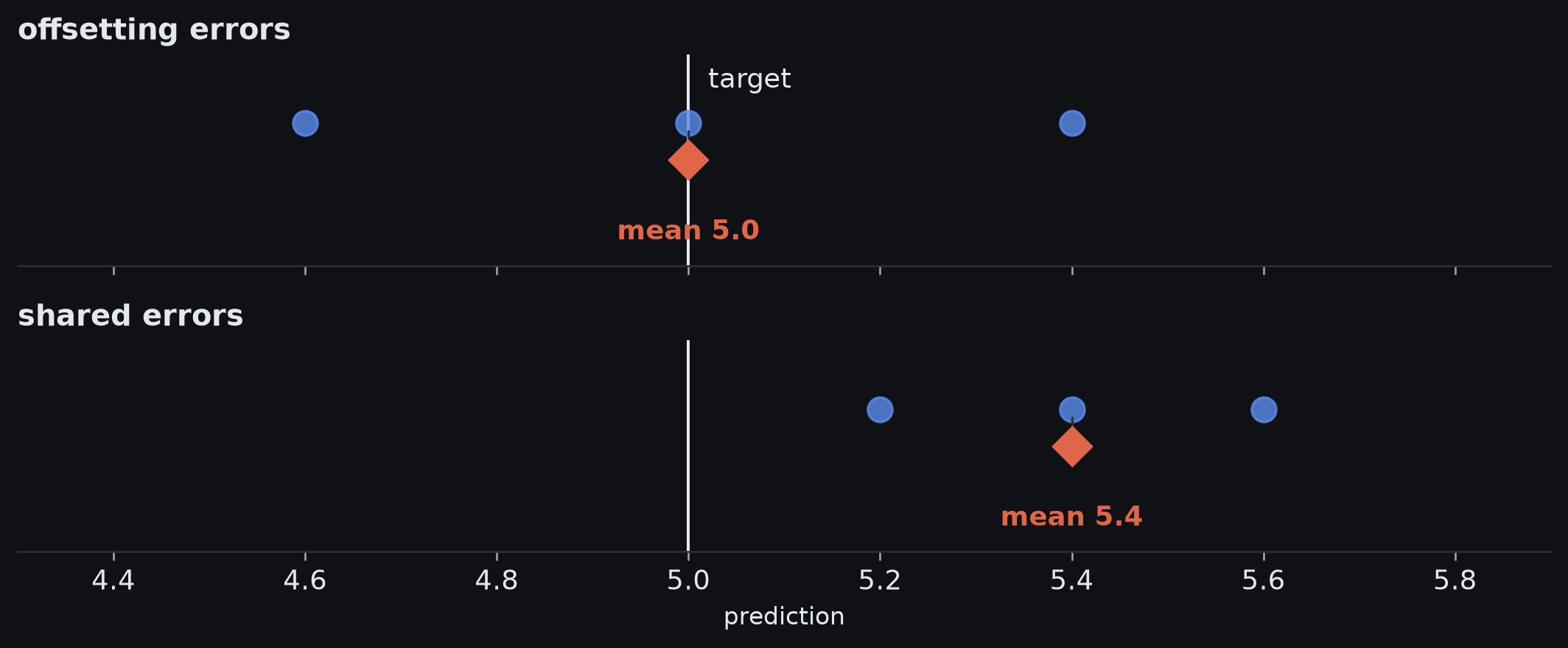
Offsetting and shared errors
Three predictions of a target of 5. Top: the errors fall on both sides and the mean lands on the target. Bottom: every error has the same sign, and the mean inherits it.
Ensembles
Definition 6 An ensemble is a group of models whose predictions are combined into one prediction.
Regression: mean or median of the outputs
Classification: mean of the pre-softmax activations, or the most frequent predicted class
The gain comes from diversity among the models’ errors.
storing the same model several times gains nothing
Correlated errors
Shared error: every model errs the same way, and averaging preserves it
Sources of diversity:
different random initialisations
different sampled datasets
different hyperparameters
different model families
Idealised case: independent errors, where the cancellation argument is strongest
Diversity from initialisation
networks started from different random parameters can converge to different fitted functions
Where it matters: regions the training data barely constrain
e.g. far from the training examples
averaging several independently trained networks moderates their arbitrary behaviour there
Bagging
Definition 7Bootstrap aggregating, or bagging, trains each model of an ensemble on its own resample of the training data, drawn with replacement, and combines their predictions.
sample a new training set with replacement from the original data
train a separate model on each resample
combine their predictions
With replacement:
some examples appear several times
some examples are absent from a particular resample
Bagging and outliers
Omitted point: a model whose resample lacks an unusual point infers that region from the remaining observations
Averaged: the ensemble is less sensitive to that one observation
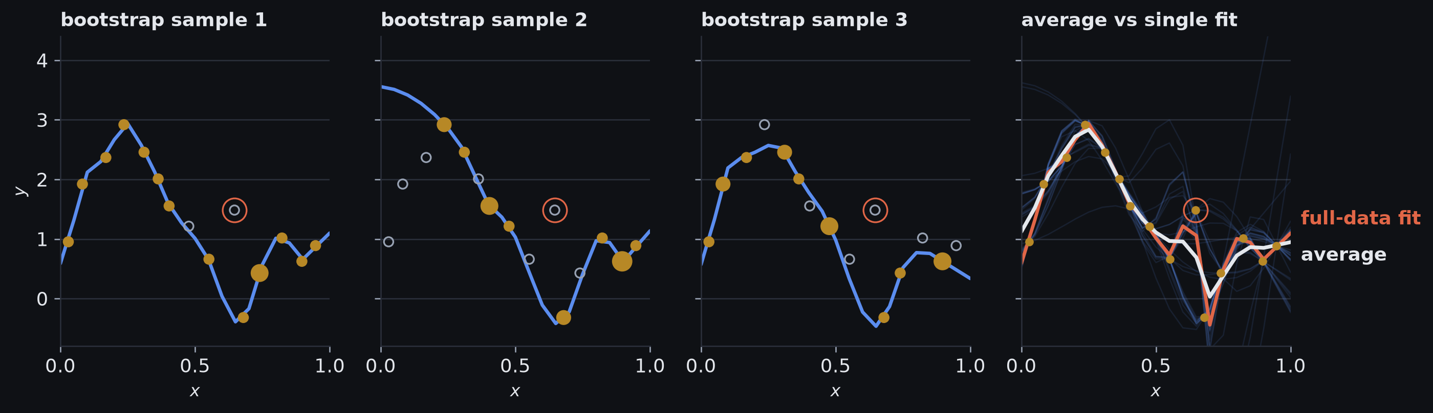
Bagging on the toy regression
Bagging on a toy regression with one unusual point (circled). The first three panels are bootstrap samples: marker size shows how many times each point was drawn, and hollow markers were not drawn at all. The last panel overlays all forty bootstrap fits, their average, and the single fit to the full data; at the unusual point the average is pulled less far from the true mean.
The cost of ensembles
multiple training runs
multiple stored parameter sets
multiple inference passes
Dropout, perturbations, and soft targets
Changing subnetworks break fragile dependencies
A network can rely on fragile partnerships between units:
one unit creates a feature
another cancels or corrects it
the combination fits the observed data
none of the units needs to work robustly on its own
A fixed smaller network would reduce capacity, but it would not create dropout’s changing-subnetwork pressure
A changing random subnetwork repeatedly breaks those partnerships, forcing useful behaviour to survive under many combinations of active units
Dropout
Definition 8Dropout clamps a random subset of hidden units to zero at each training iteration, drawing a fresh subset every time.
Tempting reading: dropping half the units just trains a smaller network
What it misses: the dropped subset changes every iteration
the active subnetwork keeps changing
all the subnetworks share the same underlying parameters
The dropout mask
Drop probability\(p\): the probability that a unit is dropped
PyTorch’s p means the same
Mask\(\vect{m}\): one entry per unit, the same shape as \(\vect{h}\)
\(m_j=1\) (kept) with probability \(1-p\), and \(m_j=0\) (dropped) otherwise
i.e. \(m_j\sim\operatorname{Bernoulli}(1-p)\)
drawn independently for each unit, afresh at each iteration
Masked activation: \(\widetilde{\vect{h}}=\vect{m}\odot\vect{h}\), the elementwise product
a dropped unit’s incoming and outgoing contributions vanish for that iteration
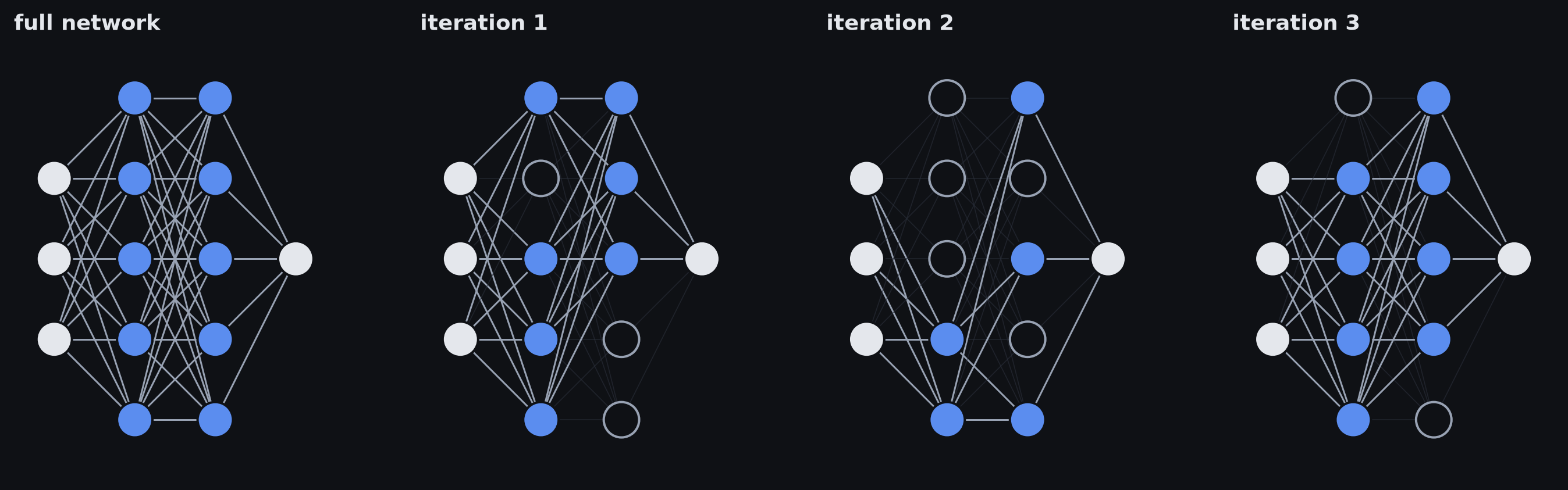
Masks across iterations
One network, four training iterations. Each iteration samples a fresh mask; dropped hidden units (hollow) take their incoming and outgoing connections with them. Every subnetwork uses the same underlying weights, so each update trains part of one shared model.
Brittle cancellation
Setup: several hidden units cooperate to build a local hinge
in a region with no training observations
so the training loss doesn’t change
Why no gradient: the hinge costs nothing, so gradient descent has no reason to remove it
What dropout does: drops one of the cooperating units
the cancellation fails, exposing the dependence
the resulting gradient pushes toward a less brittle solution
Dropout and a hidden bump
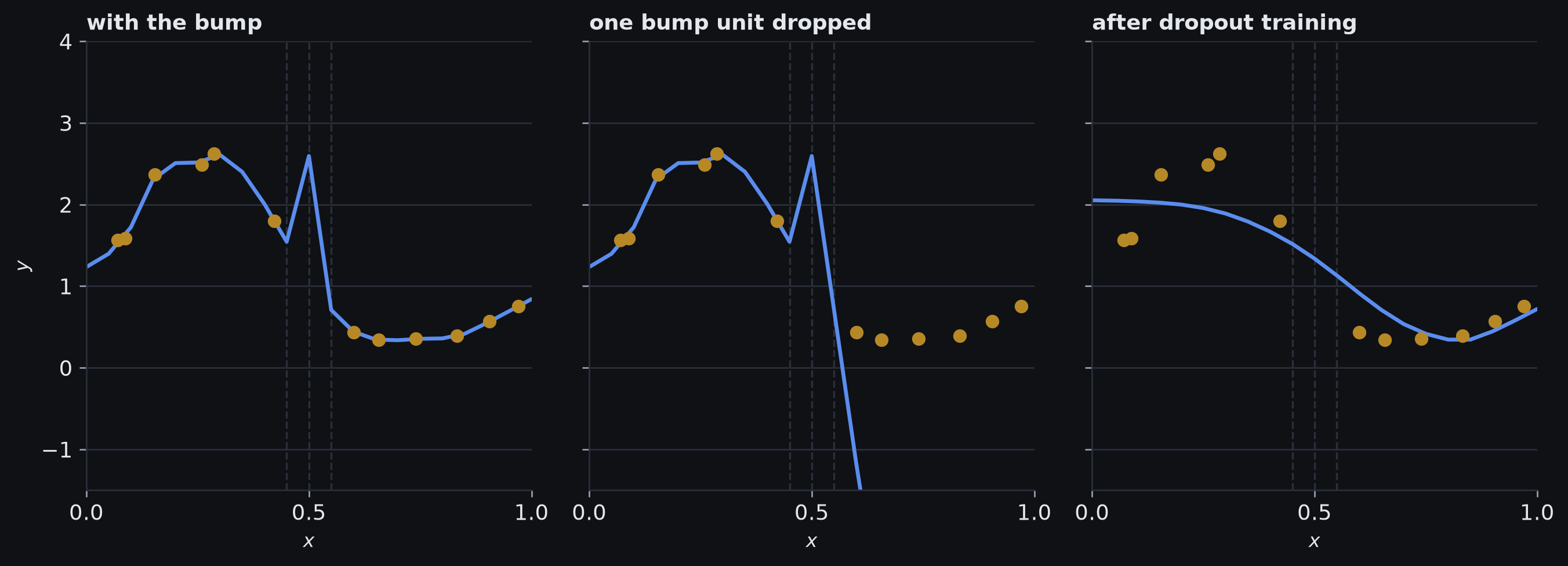
Left: a fit whose three hidden units at the dashed joints build a bump in a gap between the training points; they cancel exactly everywhere else, so the bump costs no training loss. Centre: drop one of the three and the cancellation fails, and the function moves far from the data. Right: after training with dropout, the bump’s weights have shrunk and the gap is spanned smoothly, at the cost of a looser fit to the data everywhere. The same training without dropout leaves the bump in place.
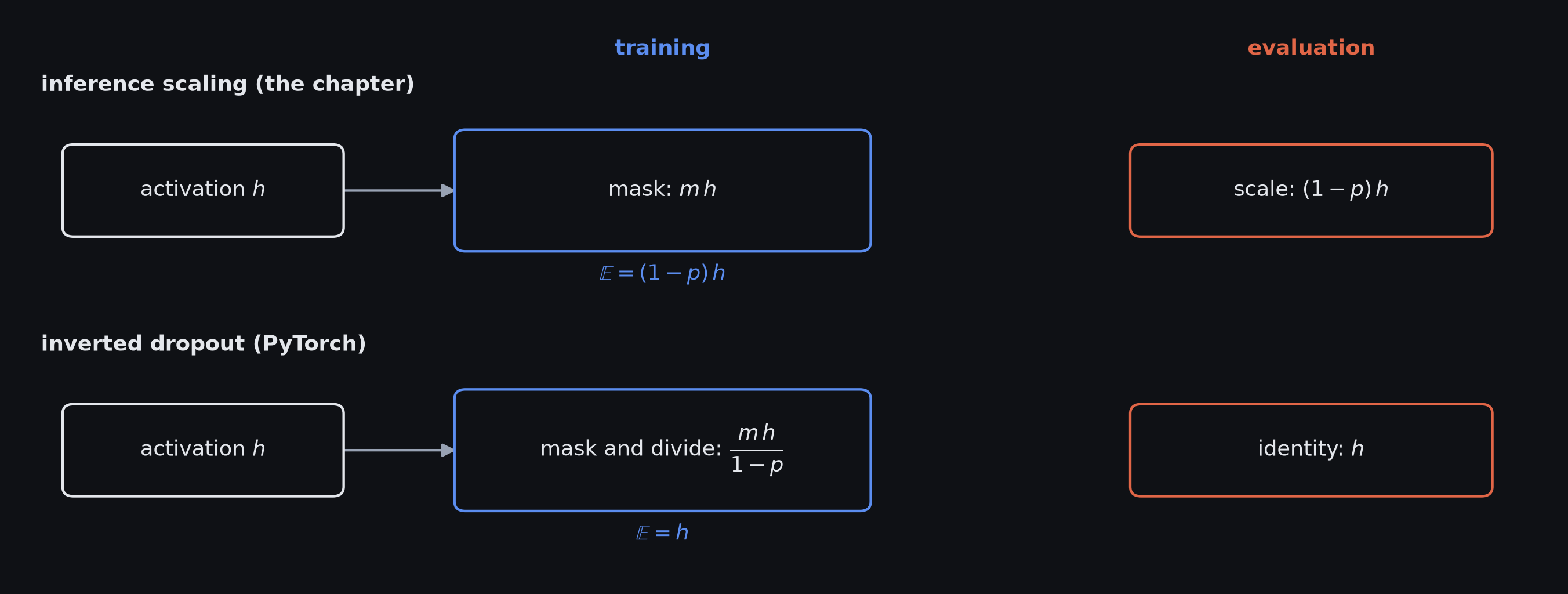
At evaluation: nn.Dropout is the identity operation
Two dropout conventions
The same activation h and drop probability p under both conventions. Top, inference scaling: training only masks, so a unit’s expected output is (1 − p)h, and evaluation multiplies by 1 − p to match. Bottom, inverted dropout, as PyTorch implements it: training masks and divides by 1 − p, so the expectation is already h and evaluation is the identity.
Inverted dropout’s expected scale
Setup: \(h=2\), \(p=0.5\), inverted dropout
Try it: what is \(\expect{\widetilde h}\)?
Dropped: value \(0\), with probability \(0.5\)
Kept: value \(2/(1-0.5)=4\), with probability \(0.5\)
\[
\expect{\widetilde h}
=0.5(0)+0.5(4)=2=h.
\]
the training activation has the same expected scale as the evaluation activation
Monte Carlo dropout
Standard inference: dropout’s randomness is switched off
Monte Carlo dropout keeps it on:
sample a dropout mask and predict
repeat several times
combine the predictions
Relation to ensembles: an ensemble-like prediction without storing separately trained networks
Dropout as multiplicative noise
a Bernoulli mask is multiplicative noise on the hidden activations
Other places to perturb:
inputs
weights
hidden activations
labels
Common question: should the desired prediction stay stable under that perturbation?
Input noise
Perturbed input: at each step, replace \(\vect{x}\) with
\[
\widetilde{\vect{x}}
=
\vect{x}+\noise.
\]
Assumption: nearby inputs should have similar outputs
Effect: fitting many perturbed copies discourages sharp local changes in the learned function
Input noise and the input Jacobian
Remember how the Jacobian collected all the first-order sensitivities of one vector to another?
In week 2 we differentiated network outputs with respect to the parameters
Here we ask a different sensitivity question: how much does the output move when the input moves?
Regression: input-noise training can be related to a regularisation term that penalises these derivatives
large input Jacobian: a small perturbation can change the prediction substantially
Input noise on the toy regression
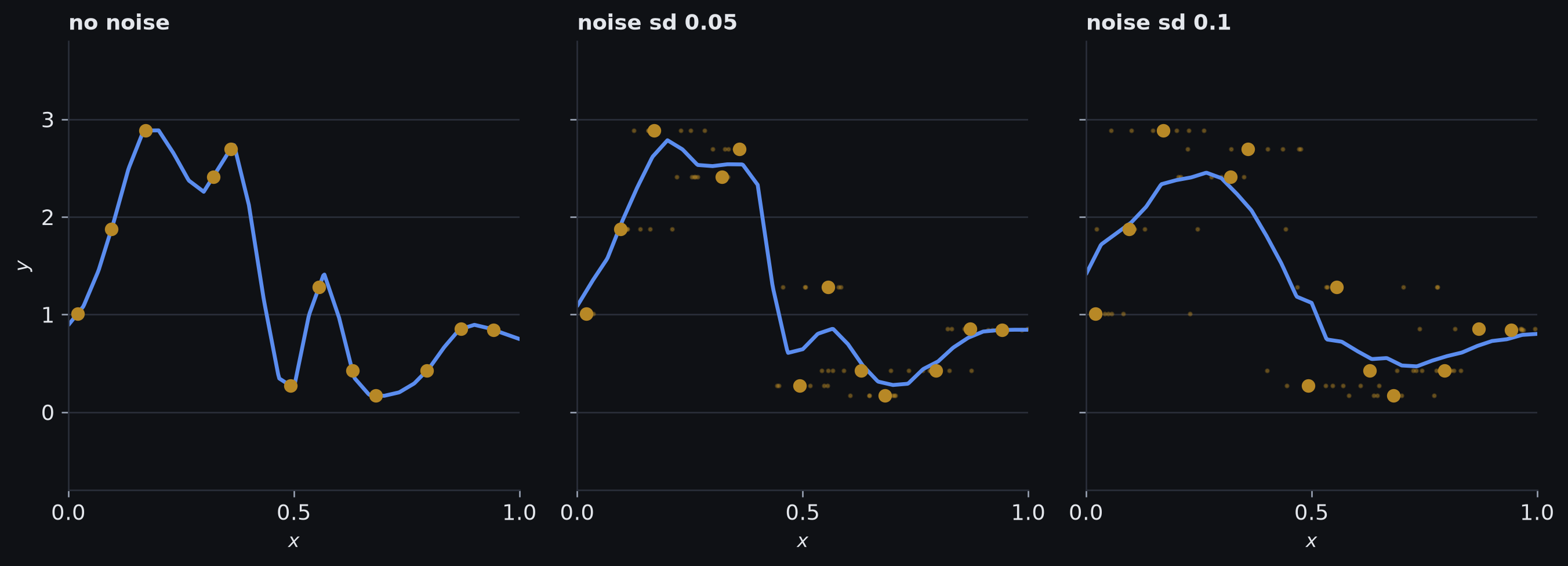
The same twelve observations and the same thirty-joint model, fitted to many perturbed copies of each input. The faint dots are some of those copies. With no noise the fit interpolates; as the noise standard deviation grows, the fitted function gets smoother.
Weight noise
Perturbed parameters: during training, use
\[
\widetilde{\params}
=
\params+\noise.
\]
a useful solution must keep working for nearby parameter values
optimisation is pushed toward regions where small parameter errors have little effect
the intuition behind seeking wide or flat minima
Limit: a better-generalisation claim for wide minima is a hypothesis with supporting evidence, not a theorem
flatness depends on how the parameters are scaled, one reason the link is not a theorem
Narrow and wide minima
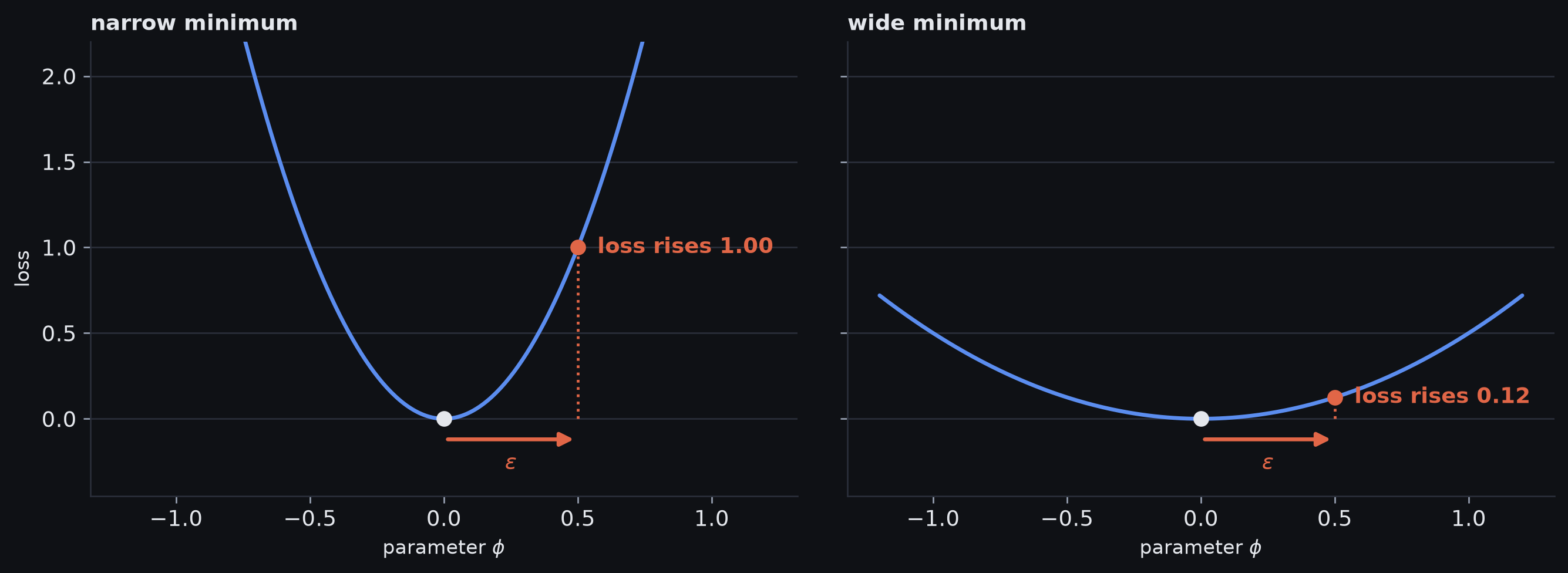
Two minima with the same loss. The same parameter perturbation ε raises the loss sharply in the narrow basin and only a little in the wide one. The link from wide minima to generalisation is an intuition with supporting evidence, not a theorem.
Adversarial training
Input noise: samples a perturbation from a fixed distribution
Adversarial training: searches for a small perturbation that causes a large change in model behaviour
a worst-case local perturbation
an extreme form of training for stability under input perturbation
Overconfident classification
One-hot target: the likelihood objective rewards pushing the labelled class’s probability toward \(1\)
Consequence: the logits are pushed toward ever more extreme values
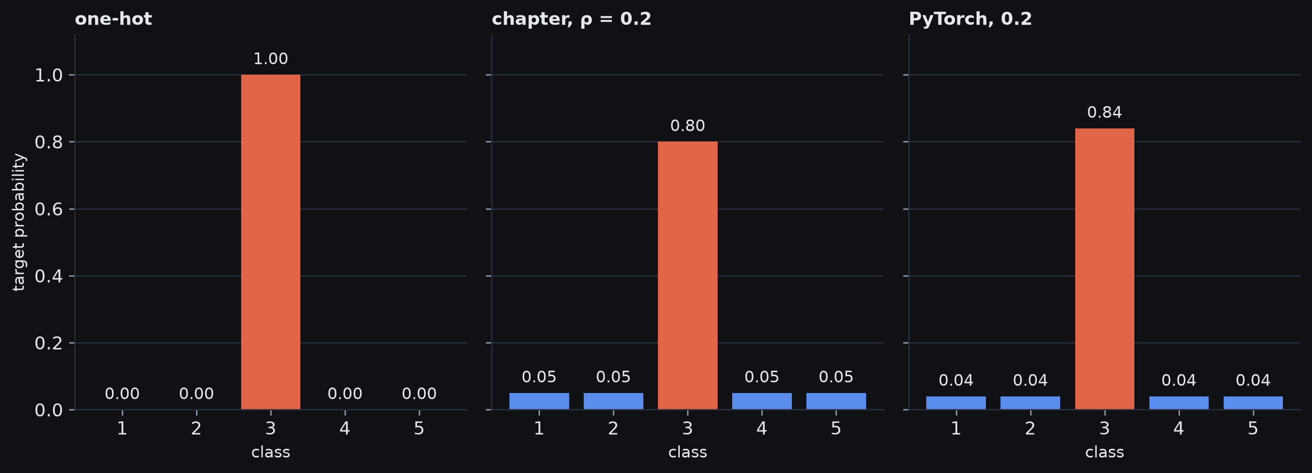
Definition 10Label smoothing replaces the one-hot target with a distribution that keeps most of the probability mass on the labelled class and spreads the rest over the other classes.
Same idea, different parameterisation: equal coefficients don’t mean equal targets
Three target distributions
The target for a five-class example whose true class is 3. Left: one-hot. Centre: the chapter’s smoothing with ρ = 0.2, which spreads ρ over the four wrong classes. Right: PyTorch’s label_smoothing = 0.2, which mixes in a uniform distribution over all five, so the true class keeps more mass.
Parameter uncertainty
One fitted parameter vector hides alternatives
Standard training usually returns one estimate \(\widehat{\params}\)
But several parameter vectors may explain the observed data almost equally well
Those alternatives can make different predictions away from the training examples
A point estimate hides that remaining uncertainty
Bayesian inference keeps a distribution over plausible parameter vectors instead of collapsing immediately to one.
This is the same motivation that made ensembles useful earlier: different plausible models can disagree
Remember maximum likelihood?
From the loss-function session, the likelihood asks
\[
p(\set{D}\mid\params):
\]
if these were the parameters, how compatible would the observed data be?
Maximum likelihood picks the single \(\params\) that makes the observed data most likely
It uses the data, but it does not represent uncertainty over which parameter values remain plausible
The likelihood answers a forward question: parameters \(\rightarrow\) possible data
The Bayesian question reverses the conditioning
For inference, the question we actually want is
\[
p(\params\mid\set{D}):
\]
after seeing these data, how plausible is each parameter vector?
\(p(\set{D}\mid\params)\) and \(p(\params\mid\set{D})\) are different quantities
We cannot simply swap the two sides of the conditioning bar
Bayes’ rule tells us how to reverse that conditioning while accounting for what was plausible before the data arrived.
Bayes as reweighting
Suppose only two candidate models are possible
candidate
prior
likelihood of observed data
prior \(\times\) likelihood
A
\(0.75\)
\(0.20\)
\(0.15\)
B
\(0.25\)
\(0.80\)
\(0.20\)
Before the data: candidate A is three times as plausible as B
Evidence from the data: the observations are four times as likely under B
Likelihood: how well a candidate explains the observations
Posterior: updated plausibility after combining both
The missing proportionality constant is the evidence that makes the posterior integrate to one
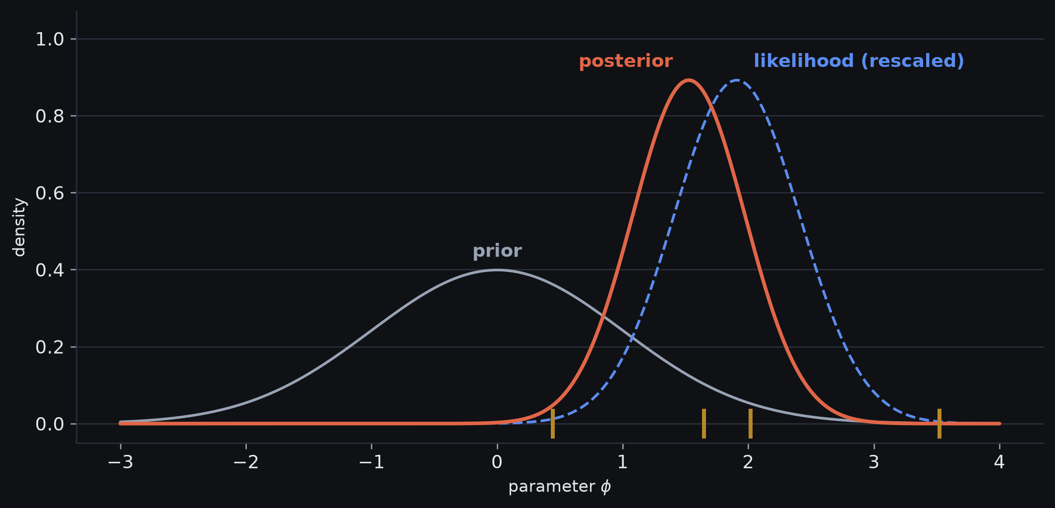
Prior, likelihood and posterior
One scalar parameter φ: the mean of four noisy observations (ticks). The prior is a Gaussian centred on 0; the likelihood peaks near the observations and is rescaled here to share the axis, since it is not a density in φ. Their product, normalised, is the posterior: between the two, and narrower than the prior.
From one parameter to a neural network
For the full parameter vector \(\params\) and training data
The evidence disappears from the \(\argmax\) because it does not depend on \(\params\)
MAP keeps one Bayesian idea: the prior can influence which fitting solution is selected
MAP discards another: uncertainty represented by the rest of the posterior
The L2 penalty has a Bayesian interpretation
Earlier, L2 was introduced geometrically:
prefer a shorter weight vector when data fit is comparable
Now ask the Bayesian version of the same modelling choice:
what prior would express a soft, symmetric preference for weights near zero?
An independent zero-centred Gaussian prior does exactly that
\[
\phi_j\sim\normal(0,\sigma_\phi^2).
\]
zero is the centre of the preference
positive and negative weights of equal magnitude are treated symmetrically
large weights remain possible, but become progressively less plausible
this is a modelling choice, not a claim that trained weights are literally sampled from a Gaussian
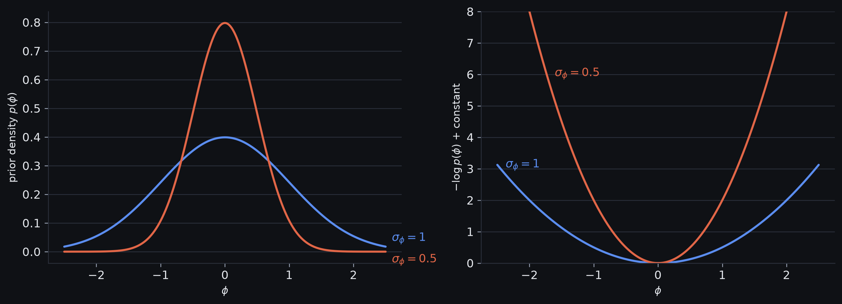
A Gaussian prior and its negative log
A zero-centred Gaussian prior and the penalty it implies. Left: smaller prior variance concentrates more density near zero. Right: taking the negative log turns each Gaussian into a quadratic bowl; the narrower prior gives the steeper penalty.
Definition 12 The posterior predictive distribution averages the prediction from every parameter vector, weighted by its posterior density.
Bayesian prediction as an ensemble
Members: every candidate \(\params\) defines a model prediction \(\Pr(y\mid\vect{x},\params)\)
Weights: posterior density \(p(\params\mid\set{D})\)
Combination: the integral is an infinite weighted ensemble
Contrast: the ensembles earlier today average a finite collection of separately fitted networks
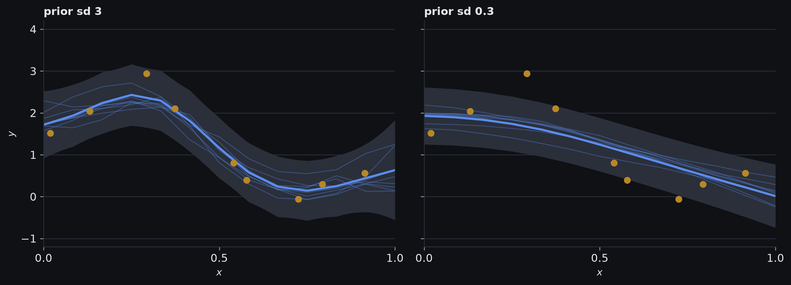
Posterior samples and the predictive band
Bayesian inference for the fixed-joint model with a Gaussian prior on its weights, computed in closed form. Thin lines are the functions given by weight vectors drawn from the posterior; the thick line is the predictive mean and the band two predictive standard deviations. Left, a broad prior: the functions follow the data and spread furthest at the right-hand end. Right, a narrow prior: the functions are held to a smoother trend, agree with one another, and miss the peak.
Bayesian neural networks in practice
For a complex neural network:
the posterior over all parameters has no general closed form
the posterior predictive integral cannot generally be evaluated exactly
Practical approximations include:
variational Bayes
Markov chain Monte Carlo
stochastic-gradient MCMC variants
Trade-off: explicit parameter uncertainty, at substantial computational and modelling cost
Additional training signal
Borrowing signal from other data
Problem: the target task has little labelled data
Source: other data supply a representation, before or alongside target-task fitting
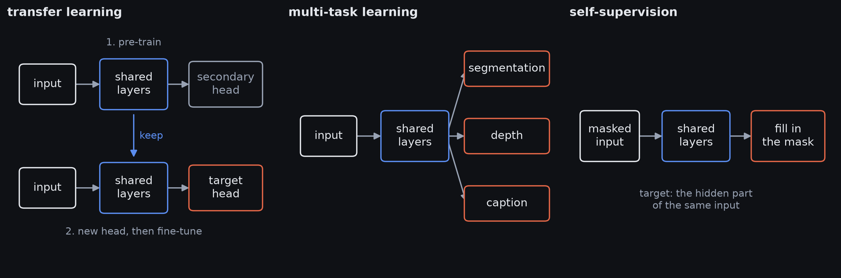
Three routes:
transfer learning
multi-task learning
self-supervised learning
Transfer learning
pre-train on a related task with more data
remove or replace the task-specific output layer
attach a head for the target task
train only the new head, or fine-tune some or all of the network
Representation view: reuse features learned on the related task
Optimisation view: start from a parameter region already shaped by that task
Freezing vs fine-tuning
Freeze the backbone: fit only the new output layers
assumes the learned representation already transfers
Fine-tune: let the representation itself adapt to the target task
Deciding factors:
volume of target data
similarity of the two tasks
cost of changing the pre-trained representation
Multi-task learning
Setting: one network learns several related objectives at once
Example, from one image:
segmentation
pixel-wise depth
a caption
Shared representation: every task needs some understanding of the same input
so each objective may benefit from the others
Generative self-supervision
Task: hide part of an example, predict the missing content
Examples:
masked image region: inpaint it
masked text token: predict it
Target source: the input itself
so large unlabelled datasets become training material
Contrastive learning
Task: compare examples that should be related with examples that should not
no reconstruction of missing content
Examples:
transformed versions of one image vs unrelated images
consecutive sentences vs unrelated sentences
spatially related patches of one image
Signal: which examples should share structure, with no human class label
Transfer, multi-task and self-supervised learning
One visual grammar for three ways to borrow training signal: a shared representation (blue) with task-specific heads. Transfer learning trains on a secondary task, then replaces the head. Multi-task learning trains several heads at once. Generative self-supervision masks part of an unlabelled input and trains the network to fill it in.
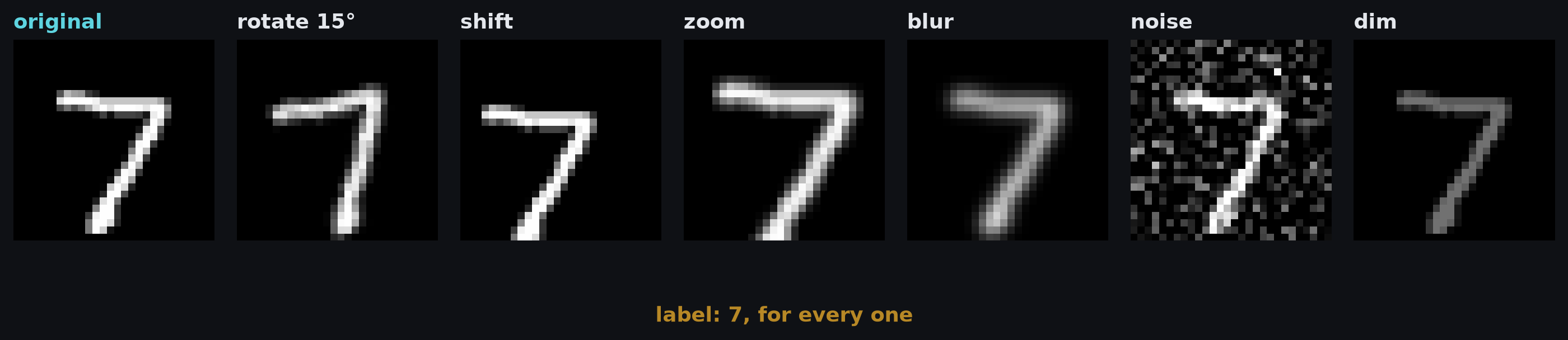
Data augmentation
Setting: an image labelled bird, for ordinary bird classification
Label-preserving transformations:
modest rotation
horizontal flip
blur
colour changes
Effect: the model learns insensitivity to variation declared irrelevant to the task
Augmentation as an assumption
Condition: useful only when the correct target stays unchanged
Pick a task: name one transformation that would break its label
Failure cases:
horizontal flip for text or asymmetric symbols
large crop that removes the labelled object
colour change when colour determines the class
word substitution that changes sentence meaning
Augmentation asserts an invariance; it does not create truth.
Multi-task learning: additional labels on related tasks
Self-supervision: targets generated from unlabelled data
Augmentation: task-preserving transformations of existing examples
Shared mechanism: constrain the representations and predictions to fit a wider body of evidence
Choosing a regularisation strategy
Mechanisms of regularisation
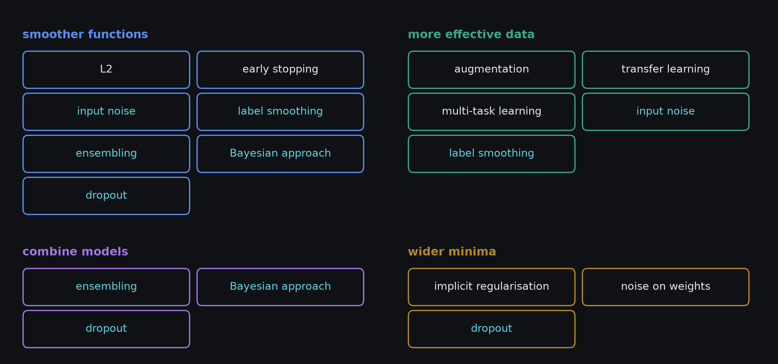
The methods can be grouped by how they improve generalisation
Smoother functions: bias the fit towards a function that changes slowly
More effective data: add examples, or information, the fit can use
Combining models: average over several fits to reduce fitting uncertainty
Wider minima: prefer a minimum where small parameter errors matter less
Methods by mechanism
Four broad regularisation mechanisms and representative methods. Methods highlighted in cyan act through more than one mechanism: input noise, label smoothing, ensembling and the Bayesian approach through two, dropout through three.
Methods with several mechanisms
Dropout: smoother functions, combining models and wider minima
Input noise, label smoothing: smoother functions and more effective data
Ensembling, Bayesian approach: smoother functions and combining models
Use: a reasoning aid; the groups overlap
Failure modes and interventions
observed concern
plausible intervention
highly sample-sensitive fit
L2, early stopping, bagging
brittle hidden-unit dependencies
dropout
sensitivity to small input changes
input noise, adversarial training
overconfident class probabilities
label smoothing
limited labelled target data
transfer, self-supervision, augmentation
uncertainty across plausible fitted models
ensemble, Bayesian treatment
Status: each row is a hypothesis to validate
Choosing the strength
Each method brings a hyperparameter
L2 coefficient \(\lambda\)
dropout probability \(p\)
stopping time
noise scale
label-smoothing strength
augmentation strength and frequency
More regularisation is not monotonically better
Right amount depends on: data, architecture, optimiser and task