Lecture 6: Measuring Performance

Week 3 · principles

Eoin O’Brien

Generalisation

Perfect on the data it has seen

Suppose a classifier reaches 100% training accuracy.

What can we conclude about a new example drawn tomorrow?

• it will probably be classified correctly
• the model has enough capacity to fit the training data
• the optimiser worked
• nothing, until we measure performance on unseen data

Ask for a vote before revealing the options. Collect explanations for a training/held-out gap without correcting them yet. Listen for: “that is overfitting”, “the optimiser failed”, “we need more data”, and “there must be a bug”.

Training fit vs held-out performance

• Training asks: how well did the model fit examples used to choose its parameters?
• Evaluation asks: how well does the fitted model behave on new examples from the task?
• A sufficiently flexible network can often fit its training set almost perfectly
• Perfect fit therefore does not establish that the learned rule extends beyond those examples

Generalisation is the extent to which performance carries from the training data to unseen data drawn from the relevant distribution.

Keep the distinction statistical rather than moral: low training error is not itself bad.

MNIST: handwritten digit classification

MNIST is a classic machine-learning benchmark for recognising handwritten digits.

• each example is a \(28\times28\) grayscale image
• the target is one of 10 digit classes: \(y\in\{0,1,\ldots,9\}\)
• the standard dataset contains 60,000 training images and 10,000 test images
• the task is simple to state: given the pixels, which digit was written?

MNIST became useful because it provided a standard, easy-to-understand classification problem on which learning methods could be compared.

MNIST-1D

MNIST-1D is a synthetic, one-dimensional analogue of MNIST.

It is not a flattened or compressed MNIST image.

• there are still 10 classes analogous to digits \(0,\ldots,9\)
• each class begins from a characteristic 1D template
• random padding, translation, scaling and noise create different examples
• each final input is a sequence of only 40 values

Instead of recognising a digit from a \(28\times28\) image, the model recognises a class from the shape of a short 1D signal.

From MNIST to MNIST-1D

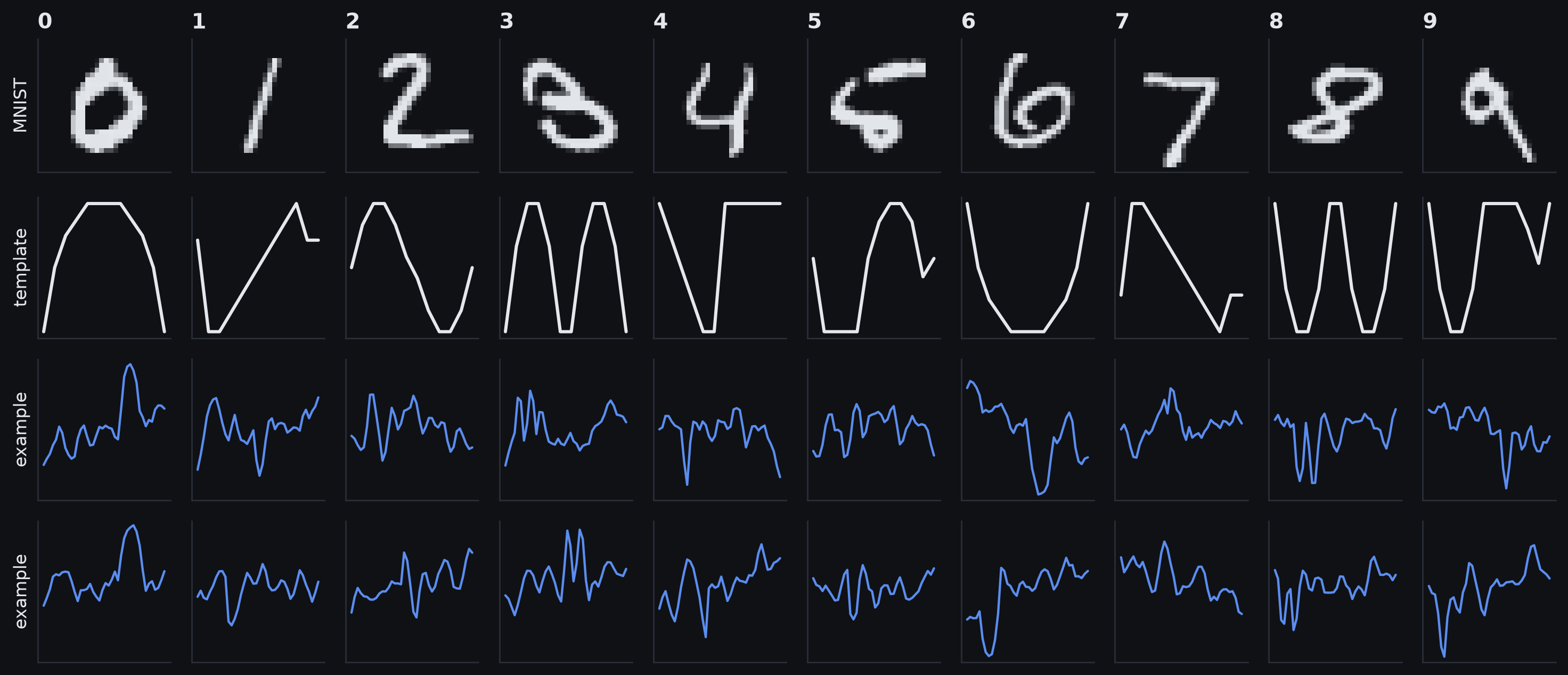
Top: one handwritten MNIST test image of each digit, 28 × 28 pixels. Second row: the ten MNIST-1D templates, the whole vocabulary of the 1D dataset. Below each, two MNIST-1D training examples of that class, each a sequence of 40 values – all the network is given. MNIST images © Yann LeCun and Corinna Cortes, CC BY-SA 3.0.

Why use MNIST-1D here?

We want to experiment with generalisation, not merely report one benchmark score.

MNIST-1D is useful because it is:

• small: the default dataset has 4000 training examples
• low-dimensional: each input contains only 40 values
• fast to train: we can repeat experiments and sweep capacity cheaply
• controllable: the data are generated procedurally, so transformations and label noise can be varied
• informative for comparison: evaluation scores are not all clustered near ceiling performance

Treat it as a laboratory: change one part of the learning problem and observe what happens to training and generalisation.

Our first MNIST-1D experiment

We begin with:

• \(I=4000\) training examples
• 40 input values per example
• two hidden layers with 100 units each
• 10 logits followed by softmax
• SGD with batch size 100 and learning rate \(0.1\)
• 6000 optimisation steps

Reminder: softmax and cross-entropy

The network produces 10 logits. Softmax converts them into 10 class probabilities.

Cross-entropy rewards assigning more probability to the correct class.

Training fit becomes perfect

After roughly 4000 optimisation steps,

\[ \text{training classification error}=0. \]

The network correctly classifies every training example.

But that is not yet the question we care about:

What happens on new examples generated by the same process?

Held-out evaluation

The fitted model has already had access to the training examples through optimisation.

A separate held-out set measures behaviour on examples that did not choose the model parameters.

For the MNIST-1D experiment:

• 1000 additional examples are generated by the same process
• training error falls to \(0\%\)
• held-out evaluation error falls only to about \(40\%\)
• uniform random guessing on 10 balanced classes gives \(90\%\) expected error

An error near \(40\%\) is far below the \(90\%\) random-guessing baseline, but still far above the \(0\%\) training error.

This establishes that training fit and generalisation are different measurements. It does not yet tell us why the gap exists.

The source notebook calls these examples a test set. Because we repeatedly inspect this curve, they are functioning pedagogically as an evaluation set rather than an untouched final test set. Reserve “test set” later for the final post-selection estimate.

Training and held-out curves

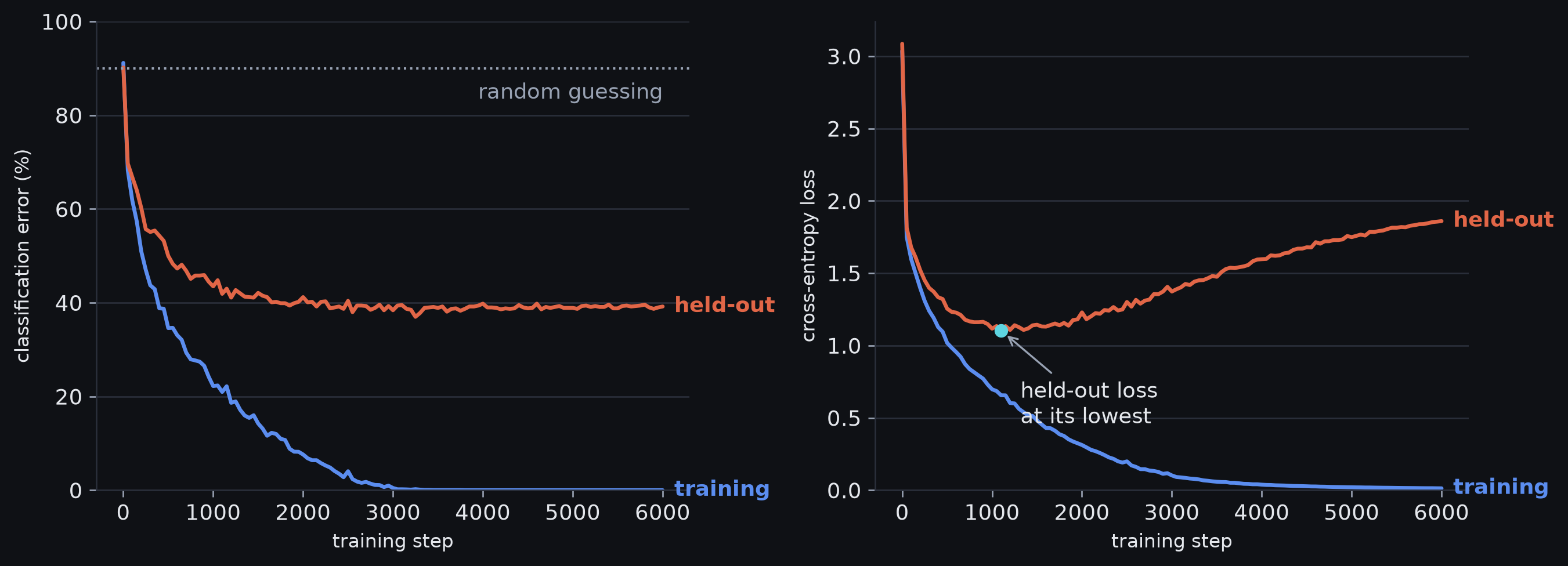
The same run scored two ways on two datasets. Left: classification error. Right: cross-entropy loss. Blue is the training set, coral the held-out evaluation set.

Error rate vs loss

For multiclass classification:

• error rate asks whether the most probable class is correct
• cross-entropy loss also cares about the probability assigned to the correct class

Recall: what cross-entropy notices

For one labelled example, \(\loss_i=-\log p(y_i\mid\vect{x}_i)\).

So cross-entropy distinguishes how much probability the model assigns to the true class even when the predicted class itself does not change.

For a three-class problem with true class A:

\(p(A)\)	\(p(B)\)	\(p(C)\)	predicted class	\(-\log p(A)\)
\(0.20\)	\(0.60\)	\(0.20\)	B	\(1.61\)
\(0.05\)	\(0.80\)	\(0.15\)	B	\(3.00\)
\(0.005\)	\(0.900\)	\(0.095\)	B	\(5.30\)

The classification error is unchanged, but the model becomes increasingly confident in the same wrong class.

Held-out loss can rise while held-out error changes little

In the MNIST-1D run:

• held-out cross-entropy initially decreases
• after roughly 1,100 steps it begins to rise
• held-out classification error changes much less

Classification error changes little, while wrong predictions can receive increasingly extreme probabilities.

The logits — the pre-softmax activations — become increasingly extreme as training pushes the probability of the correct training labels towards one.

Reconnect to Chapter 5: NLL sees confidence; 0/1 error discards it. Do not call the two metrics interchangeable.

A training/held-out gap has several possible causes

A large gap can be consistent with:

• limited or noisy training data
• a model whose flexibility interacts badly with the sample
• model choices tuned against the wrong data
• a distribution mismatch between training and held-out data
• a software or data-processing defect

The gap is evidence to investigate, not a diagnosis by itself.

Return to the explanations collected on the opening slide. Do not diagnose the gap as overfitting from this evidence alone.

Noise, bias, and variance

Why switch to a toy regression problem?

MNIST-1D showed us that a generalisation gap can exist. It did not tell us what produced that gap.

To separate possible causes, move temporarily to a synthetic 1D regression problem where we control the data-generating process:

• \(x\in[0,1]\)
• a fixed underlying quasi-sinusoidal mean function
• Gaussian noise with fixed variance, centred on that mean function
• training and fresh evaluation examples drawn independently from the same process

Now we know the underlying mean, choose the noise process, and can repeatedly draw new training datasets. That lets us isolate noise, bias, and variance rather than merely observe one aggregate error.

The toy data

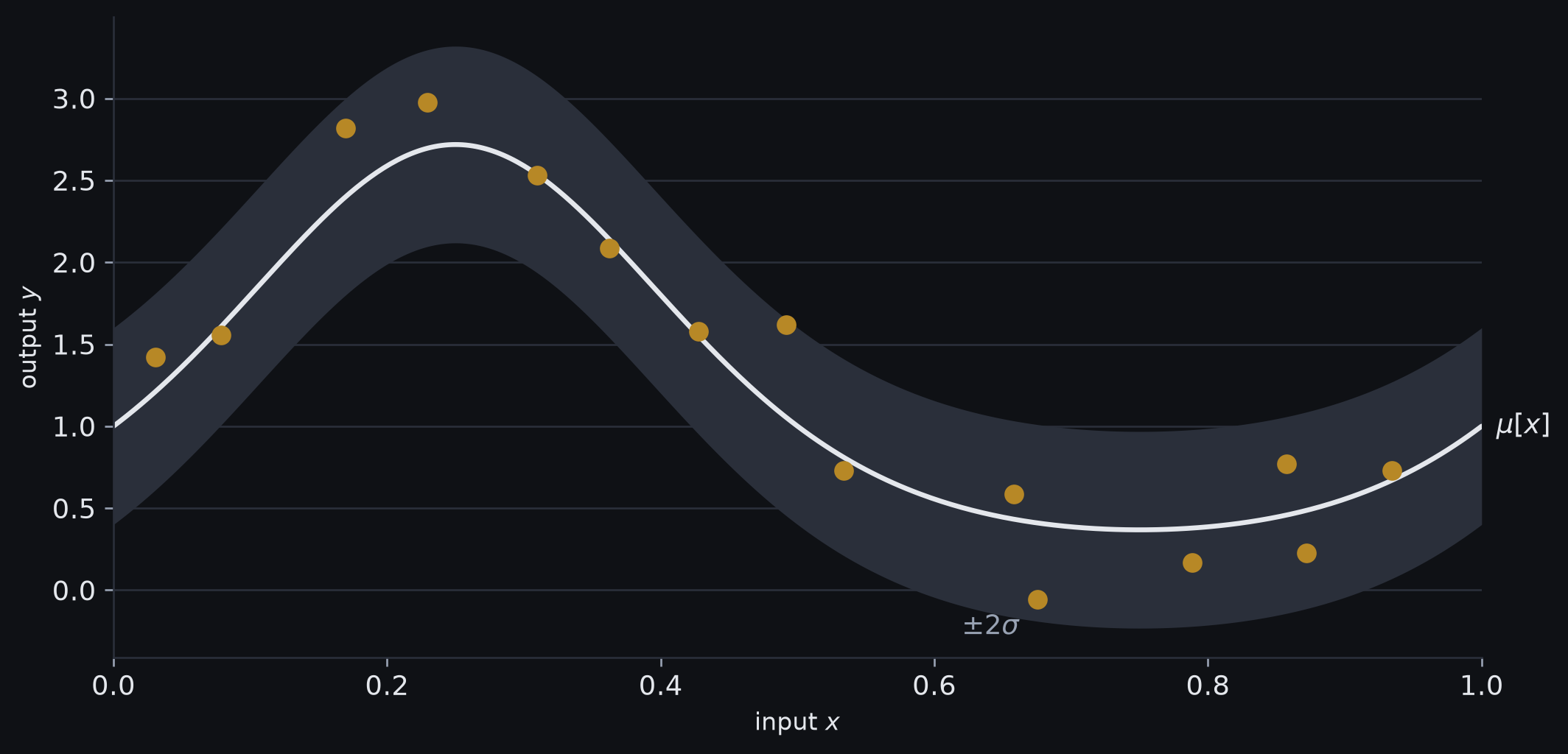
The mean function (ink), a band of two noise standard deviations either side of it, and one training set of noisy observations. Repeated outputs at the same input would scatter across the band, so even the mean itself misses them.

Fixed joints

A joint is a point where a piecewise-linear function can change slope.

The simplified network fixes these joints at regular positions. With \(D\) hidden units, they occur at

\[ 0,\frac{1}{D},\frac{2}{D},\ldots,\frac{D-1}{D}. \]

Changing the remaining parameters produces a piecewise-linear function with \(D\) regions over \([0,1]\).

With these input-to-hidden parameters fixed, the remaining fitting problem has a closed-form solution.

That lets the experiment reach the global least-squares minimum directly, so changes in error can be attributed to data and capacity rather than stochastic optimisation failure.

Three ways to miss the target

At one fixed input \(x\), prediction error can reflect three different things:

source	what varies?	intuition
noise	the observed \(y\)	valid outputs differ even when \(x\) is fixed
bias	the average fitted prediction	the learning procedure systematically misses the underlying mean
variance	the fitted model	a different training sample gives a different fitted function

Bias and variance both concern the learning procedure across possible training datasets; variance is the spread around the average fitted predictor, while bias is the average predictor’s systematic offset from the underlying mean.

Noise, bias, and variance

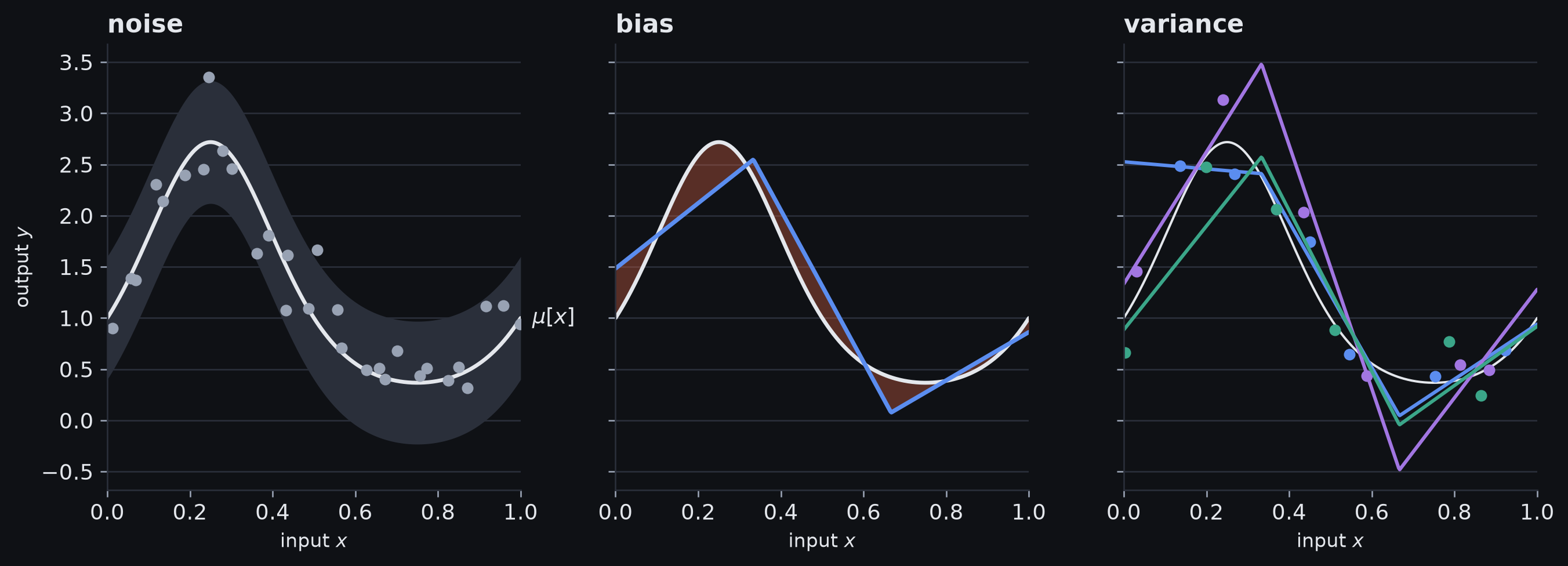
Left, noise: even the true mean misses fresh observations. Centre, bias: the best three-region fit cannot follow the mean, and the shading is its systematic error. Right, variance: fits to three different training sets of six points, each coloured with its own data.

Noise

Noise is variation in the data-generating process.

For a fixed input \(x\), there may be several valid observed outputs \(y\).

Noise can arise from:

• genuine randomness
• label or measurement error
• relevant variables that were not observed

Even a model that exactly recovers the conditional mean can still incur prediction error because the next observation is noisy.

Noise also need not prevent an extremely flexible model from fitting the training examples: if each input is observed only once, the model can memorise the particular noisy target it saw.

Irreducible here means irreducible given the observed input representation and the assumed task distribution.

Bias

Formally, bias compares the average fitted predictor across possible training datasets with the underlying conditional mean.

The toy model makes one important source of bias especially visible: even with abundant data and optimal fitting, a three-region piecewise-linear family cannot exactly reproduce the quasi-sinusoidal ground truth.

This is approximation bias from the model family. In the formal definition used here, bias belongs to the whole learning procedure, so systematic effects of fitting can also shift the average predictor.

Stress that this is not the bias parameter in an affine layer. The same English word is doing a different job.

Variance

Train the same model family several times on independently sampled datasets of the same size.

If the fitted functions differ substantially, the learning procedure has high variance with respect to the sampled training data.

• the architecture can be identical
• the fitting rule can be identical
• only the sampled examples need to change

Stochastic optimisation can add another source of run-to-run variation in practice.

Repeated training sets

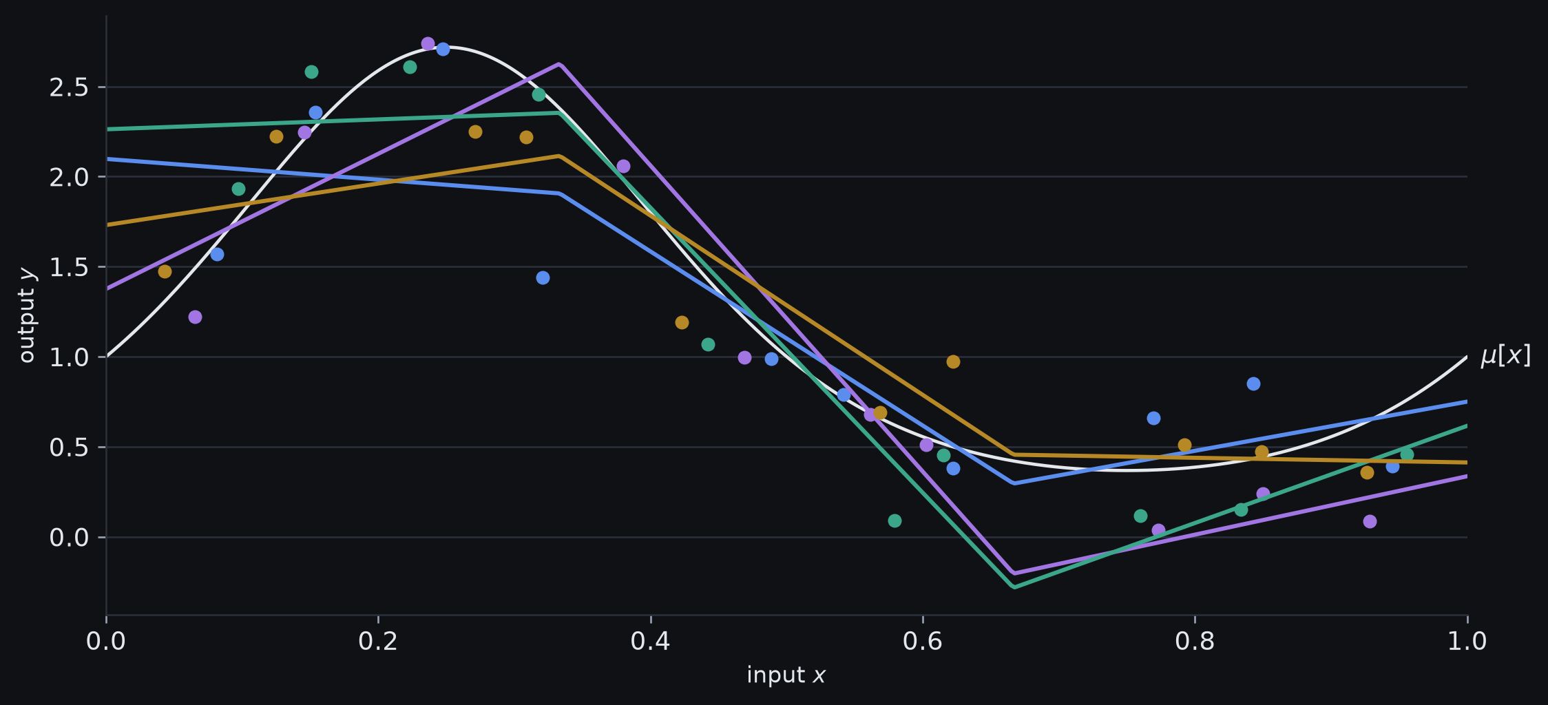
The three-region model fitted to four independently drawn training sets of ten points, each fit coloured with its own data. The model family, the fitting rule and the data-generating process are the same every time; only the sample changes.

Bias vs variance

Bias asks:

If I could average away the accidents of the training sample, where would this learning procedure predict?

Variance asks:

How much would the fitted prediction move if I drew a different training sample?

Noise asks a third question:

Even if I knew the underlying mean exactly, how much would the next observed target vary?

Why separate them?

• noise cannot be removed merely by fitting a different function to the same observed inputs
• bias points to systematic limitations of the model family or learning procedure
• variance points to sensitivity to which training examples happened to be sampled

The same overall error can therefore imply different interventions.

Bias–variance decomposition

Can the three sources be made exact?

We now have three intuitive sources of prediction error. For squared-error regression, we can ask a stronger question:

Can we show that

\[ \text{expected squared prediction error} = \text{noise} + \text{variance} + \text{squared bias}? \]

We will derive the result from two averages rather than treat it as a formula to memorise.

Expectation

For a random variable \(Z\),

\[ \expect{Z} \]

is its mean or expected value.

Reminder: expectation

Expectation is a probability-weighted average. For a continuous variable, the corresponding weighted sum becomes an integral over its density.

The subscript tells us what is being averaged over:

• \(\expectsub{y}{\cdot}\): vary the observed target at a fixed \(x\)
• \(\expectsub{\set{D}}{\cdot}\): vary the sampled training dataset

A term that does not depend on the variable being averaged can be taken outside the expectation.

Two sources of randomness enter the decomposition

At a fixed input \(x\), keep two experiments separate:

1. draw a training dataset \(\set{D}\) and fit \(\model[{\params[\set{D}]}]{x}\)
2. independently draw a fresh target \(y[x]\) from the conditional distribution at that same input

• \(\expectsub{y}{\cdot}\) varies the fresh observed target while the fitted model is held fixed
• \(\expectsub{\set{D}}{\cdot}\) varies the training sample and therefore retrains the model

The two averages

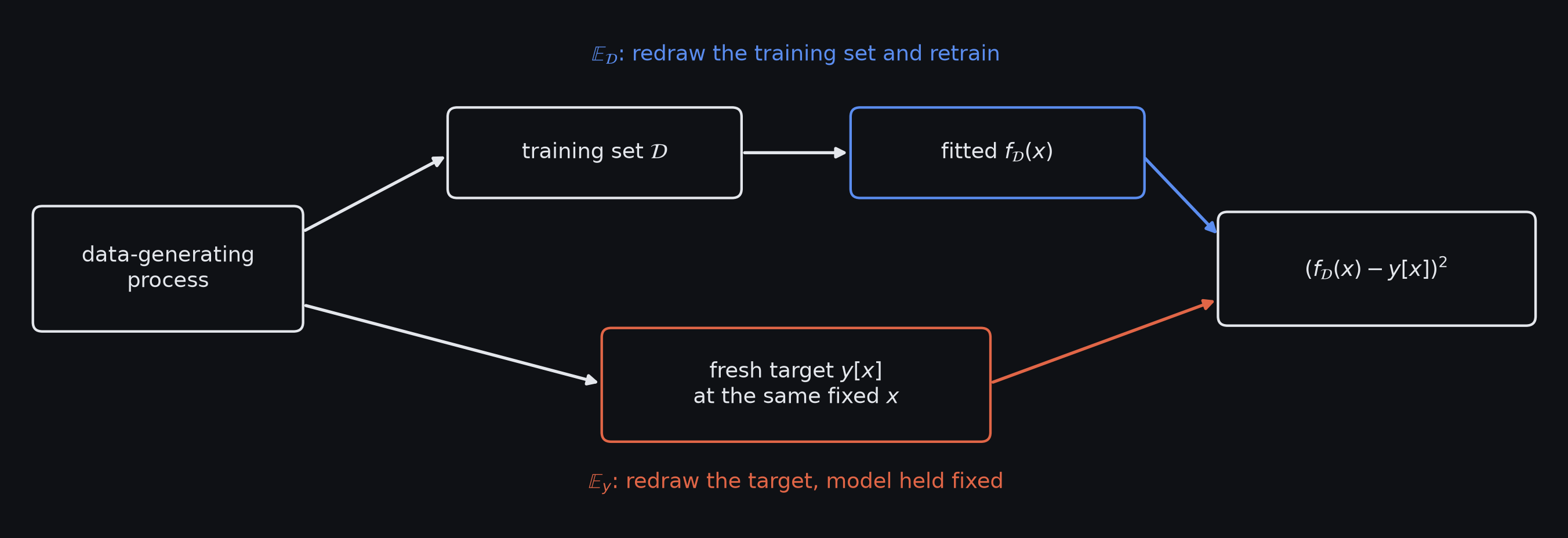
Two independent draws from the same process. The upper branch samples a training set and fits a model; averaging over it retrains the model. The lower branch draws a fresh target at the fixed input; averaging over it holds the model fixed. The loss at x needs one of each.

Fix one input before doing the algebra

Hold one input \(x\) fixed.

For continuous \(y\) with conditional density \(p(y\mid x)\), read \(p(y\mid x)\) as the distribution of possible outputs with this input held fixed, and define

\[ \mu[x] = \expectsub{y}{y[x]} = \int y[x]\,p(y\mid x)\,dy \]

as the conditional mean output at that input.

The notation \(y[x]\) emphasises that we are considering the random output at this particular input position.

Define the conditional noise variance at this input as

\[ \sigma^2[x] = \expectsub{y}{(y[x]-\mu[x])^2}. \]

The toy experiment uses a fixed Gaussian noise scale, but the decomposition itself does not require the same variance at every \(x\).

First split: prediction error plus observation noise

For one fitted model, the squared loss at \(x\) is

\[ \loss[x] = \left(\model{x}-y[x]\right)^2. \]

Reminder: squared loss

Squared loss measures the squared distance between a scalar prediction and its observed target. The square makes both positive and negative residuals contribute positively and penalises larger misses more strongly.

Add and subtract the conditional mean \(\mu[x]\):

\[ \loss[x] = \left( \underbrace{\model{x}-\mu[x]}_{\text{model versus mean}} + \underbrace{\mu[x]-y[x]}_{\text{observation noise}} \right)^2. \]

This is an exact identity.

Expanding the square

Let

\[ a=\model{x}-\mu[x], \qquad b=\mu[x]-y[x]. \]

Then

\[ (a+b)^2=a^2+2ab+b^2. \]

So

\[ \loss[x] = (\model{x}-\mu[x])^2 +2(\model{x}-\mu[x])(\mu[x]-y[x]) +(\mu[x]-y[x])^2. \]

Average over possible fresh outputs \(y\) at this fixed \(x\).

The first cross term averages to zero

Take \(\expectsub{y}{\cdot}\) while holding the fitted model fixed.

The factor \(\model{x}-\mu[x]\) does not depend on which fresh output \(y[x]\) is observed, so it leaves the expectation:

\[ \begin{aligned} &\expectsub{y}{2(\model{x}-\mu[x])(\mu[x]-y[x])}\\ &\qquad=2(\model{x}-\mu[x])\expectsub{y}{\mu[x]-y[x]}. \end{aligned} \]

By the definition \(\mu[x]=\expectsub{y}{y[x]}\),

\[ \expectsub{y}{\mu[x]-y[x]} = \mu[x]-\mu[x] =0. \]

The positive and negative observation deviations therefore cancel in expectation.

Expected loss for one fitted model

After the cross term vanishes,

\[ \boxed{ \expectsub{y}{\loss[x]} = \left(\model{x}-\mu[x]\right)^2 + \sigma^2[x] } \]

Two contributions remain:

• squared distance from the fitted prediction to the conditional mean
• observation noise

The first contribution still mixes bias and variance because the fitted model depends on which training dataset we happened to observe.

The fitted model as a random variable

Let the training dataset be

\[ \set{D}=\{(\vect{x}_i,y_i)\}_{i=1}^{I}. \]

Training on a different sample generally produces different parameters, so write

\[ \model[{\params[\set{D}]}]{x}. \]

For this derivation, hold the fitting procedure fixed and treat the learned model as deterministic once \(\set{D}\) is fixed. The outer expectation then varies the training dataset.

If optimisation itself is stochastic, run-to-run randomness adds another source of variability; it can be conditioned on separately or included in the outer averaging.

Average model prediction across datasets

Define

\[ f_\mu[x] = \expectsub{\set{D}}{\model[{\params[\set{D}]}]{x}}. \]

Read this as:

train the same procedure on every possible dataset drawn from the process, predict at \(x\), then average those predictions

We do not have to be able to perform this experiment literally for the quantity to define what bias and variance mean.

Second split: deviation around the average model

Start from the remaining model-error term

\[ \left(\model[{\params[\set{D}]}]{x}-\mu[x]\right)^2. \]

Add and subtract \(f_\mu[x]\):

\[ \left( \underbrace{\model[{\params[\set{D}]}]{x}-f_\mu[x]}_{\text{sample-specific deviation}} + \underbrace{f_\mu[x]-\mu[x]}_{\text{systematic deviation}} \right)^2. \]

Again, this is an exact identity before taking expectations.

The second cross term also averages to zero

Expand and average over possible training datasets \(\set{D}\).

The factor \(f_\mu[x]-\mu[x]\) is fixed while the dataset varies, so the cross term becomes

\[ \begin{aligned} &\expectsub{\set{D}}{2(\model[{\params[\set{D}]}]{x}-f_\mu[x])(f_\mu[x]-\mu[x])}\\ &\qquad=2(f_\mu[x]-\mu[x])\expectsub{\set{D}}{\model[{\params[\set{D}]}]{x}-f_\mu[x]}. \end{aligned} \]

But \(f_\mu[x]\) is defined as that average, so

\[ \expectsub{\set{D}}{\model[{\params[\set{D}]}]{x}-f_\mu[x]} = f_\mu[x]-f_\mu[x] =0. \]

The sample-specific deviations cancel around the average fitted prediction.

Expected squared model error

We therefore obtain

\[ \expectsub{\set{D}}{\left(\model[{\params[\set{D}]}]{x}-\mu[x]\right)^2} = \underbrace{ \expectsub{\set{D}}{\left(\model[{\params[\set{D}]}]{x}-f_\mu[x]\right)^2} }_{\text{variance}} + \underbrace{ \left(f_\mu[x]-\mu[x]\right)^2 }_{\text{squared bias}}. \]

The pointwise bias itself is \(f_\mu[x]-\mu[x]\); the loss contribution is its square.

Noise + variance + squared bias

Combining the two splits gives

\[ \boxed{ \expectsub{\set{D}}{\expectsub{y}{\loss[x]}} = \underbrace{ \expectsub{\set{D}}{(\model[{\params[\set{D}]}]{x}-f_\mu[x])^2} }_{\text{variance}} + \underbrace{ (f_\mu[x]-\mu[x])^2 }_{\text{squared bias}} + \underbrace{\sigma^2[x]}_{\text{noise}} } \]

For least-squares regression, this is the exact additive decomposition.

Noise, variance and squared bias

Noise \(\sigma^2[x]\)

• the target itself varies around its conditional mean
• changing the fitted model cannot remove this component

Squared bias \((f_\mu[x]-\mu[x])^2\)

• the average fitted model systematically misses the conditional mean

Variance \(\expectsub{\set{D}}{(\model[{\params[\set{D}]}]{x}-f_\mu[x])^2}\)

• individual fitted models move around that average when the training sample changes

If you forget the formula, reconstruct the ideas from the experiments:

1. change the fresh target at fixed \(x\) \(\rightarrow\) noise
2. change the training dataset and retrain \(\rightarrow\) variance
3. average those fitted models and compare with the true mean \(\rightarrow\) bias

Assumptions of the decomposition

The additive identity above assumes:

• regression with squared loss
• a fixed input \(x\)
• expectation over possible fresh outputs \(y\) at that \(x\)
• expectation over possible sampled training datasets \(\set{D}\)
• conditional noise variance \(\sigma^2[x]\) at the fixed input; it may vary with \(x\)

Noise, bias and variance remain useful concepts for other tasks, but they do not generally combine by this same three-term addition for arbitrary classification losses.

Do not let “bias + variance + noise” become a memorised universal equation. Ask which assumption makes the algebra work: the square and its vanishing cross terms.

Optional classification aside: noise, bias and variance remain meaningful concepts, but their effects need not combine additively under classification error. In some decision-boundary settings, additional prediction variance can even move some otherwise wrong predictions across the boundary. Do not present the least-squares identity as a universal classification formula.

Averaging over inputs gives overall expected risk

Equation 8.7 is pointwise in \(x\).

If inputs are themselves drawn from a distribution \(p(x)\), an overall expected squared error can average again over \(x\):

\[ \expectsub{x}{\expectsub{\set{D}}{\expectsub{y}{\loss[x]}}}. \]

The same three contributions are then averaged across the parts of the input space that the task actually visits. In particular, the overall noise contribution is \(\expectsub{x}{\sigma^2[x]}\).

This extra expectation is a generalisation of the fixed-\(x\) derivation, not a new fourth error source.

Capacity and overfitting

From explaining error to changing it

The decomposition tells us where expected error comes from. Now ask what we can change.

Two useful experimental levers are:

• dataset size: how many training examples we observe
• model capacity: how flexibly the learning system can fit relationships in those examples

Hold the other ingredients fixed and vary one lever at a time.

More data stabilises the fitted function

Variance comes from sensitivity to the particular sampled training set.

Holding the task and model family fixed, increasing the number of training examples usually:

• samples the input space more densely
• makes individual noisy observations less influential on the fitted function
• makes independently fitted models more similar
• reduces the variance contribution

It does not remove irreducible noise or repair a model family with substantial bias.

The same model at 6, 10, and 100 examples

In the toy experiment:

• with 6 examples, independently fitted curves differ substantially
• with 10 examples, the spread is smaller
• with 100 examples, the fitted curves are very similar

The variable being changed is dataset size, not architecture.

Six, ten, and a hundred examples

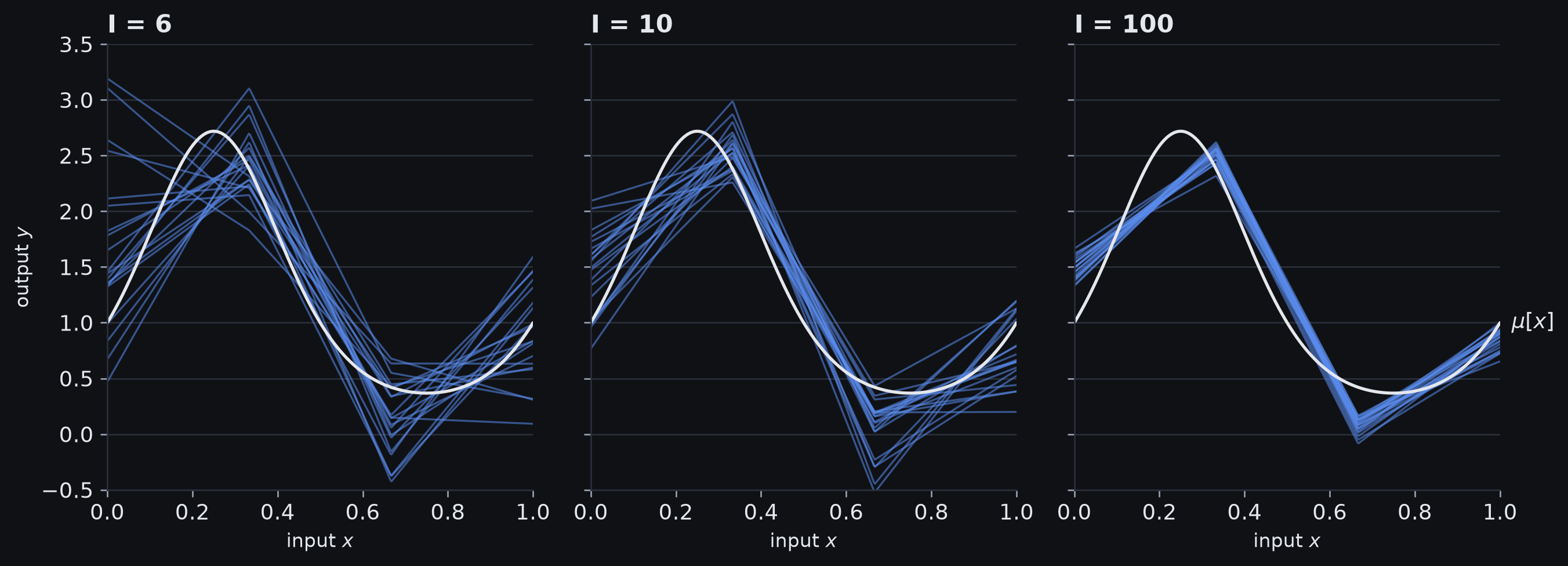
The three-region model fitted to twenty independent training sets at each size. The model family is the same in every panel; only the number of examples changes.

More capacity can reduce approximation bias

The toy model divides \([0,1]\) into piecewise-linear regions.

Adding hidden units creates more regions, so the family can represent a wider range of functions.

As capacity increases, the best attainable approximation can move closer to the underlying mean function.

That reduces bias in this example.

Capacity is about the set of behaviours the learning system can express or reach, not simply whether a network looks “large”.

Notions of capacity

Parameter count or hidden-unit count are convenient proxies, but several different notions of capacity matter:

• representational capacity: functions obtainable over all parameter settings
• effective capacity: functions the model and training procedure can actually reach
• parameter count: one rough architectural indicator of potential flexibility

Two systems with the same number of parameters can have different effective capacity because architecture, optimisation, regularisation and training time constrain what is reached.

More flexibility can increase sample sensitivity

With a fixed amount of noisy training data, a more flexible model can respond more strongly to sample-specific accidents.

In the classical regime:

• increasing capacity tends to reduce bias
• increasing capacity tends to increase variance

A lower training error therefore need not imply lower held-out error.

Overfitting

Compare two capacities on the same noisy task:

• a low-capacity model cannot follow every training point
• a higher-capacity model can fit more of their local irregularities

When that extra fit captures noise or sample-specific structure rather than the underlying relationship, held-out performance can degrade.

That behaviour is overfitting.

A training/held-out gap alone still does not tell us whether this is the cause.

The classical bias–variance trade-off

For the toy regression problem with fixed training-set size:

• bias falls as capacity increases
• variance rises
• their sum can therefore have a minimum at an intermediate capacity

In the particular toy experiment, the minimum occurs at four hidden units / linear regions.

That number belongs to the toy setup, not to neural networks in general.

Bias and variance against capacity

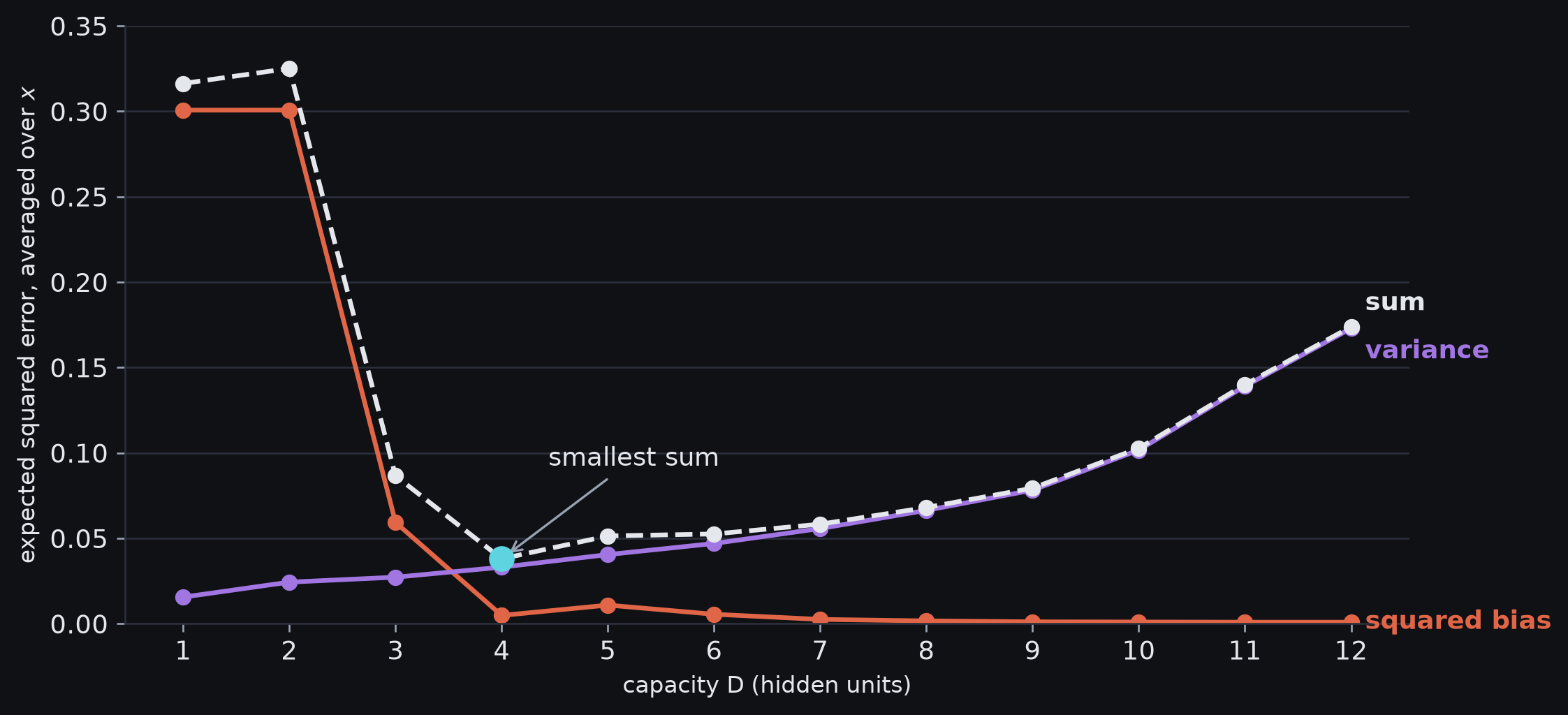
Squared bias and variance, averaged over the input range, against capacity, for training sets of 15 points; each capacity is fitted to the same 200 training sets. The fixed noise term would add the same offset at every capacity, so it does not move the minimum.

What should happen if capacity keeps increasing?

The classical bias–variance trade-off picture from the toy experiment suggests a plausible prediction:

\[ \text{too little capacity} \rightarrow \text{high bias} \rightarrow \text{best region} \rightarrow \text{high variance}. \]

If this picture were universal, once held-out error started rising, more capacity should keep making it worse.

Ask students to predict the continuation of the curve before revealing the next section.

Double descent

Test the classical prediction on MNIST-1D

The MNIST-1D capacity sweep uses:

• 10,000 training examples
• 5,000 evaluation examples
• a two-hidden-layer network
• Adam with step size \(0.005\)
• full-batch training for 4000 steps

With the original labels, evaluation error continues to decrease even after training error is essentially zero.

The classical U-shaped curve is not a universal description of neural-network generalisation.

Label noise makes the interpolation threshold easier to see

With the original labels, evaluation error keeps improving across this sweep.

To make the interpolation threshold easier to expose:

• randomise 15% of the training labels
• leave the evaluation labels unchanged

The randomised labels deliberately break the relationship between some training inputs and their assigned targets.

A model cannot infer those assignments from the underlying class structure; to drive training error to zero, it must increasingly fit these sample-specific labels too.

Double descent

As capacity increases:

1. evaluation error first decreases
2. it rises near the capacity needed to fit the noisy training set exactly
3. it then decreases again in a more highly over-parameterised regime

This is double descent.

This curve is an observation, not yet an explanation.

We still need to understand how many interpolating solutions can exist and why training reaches some rather than others.

Clean and noisy labels

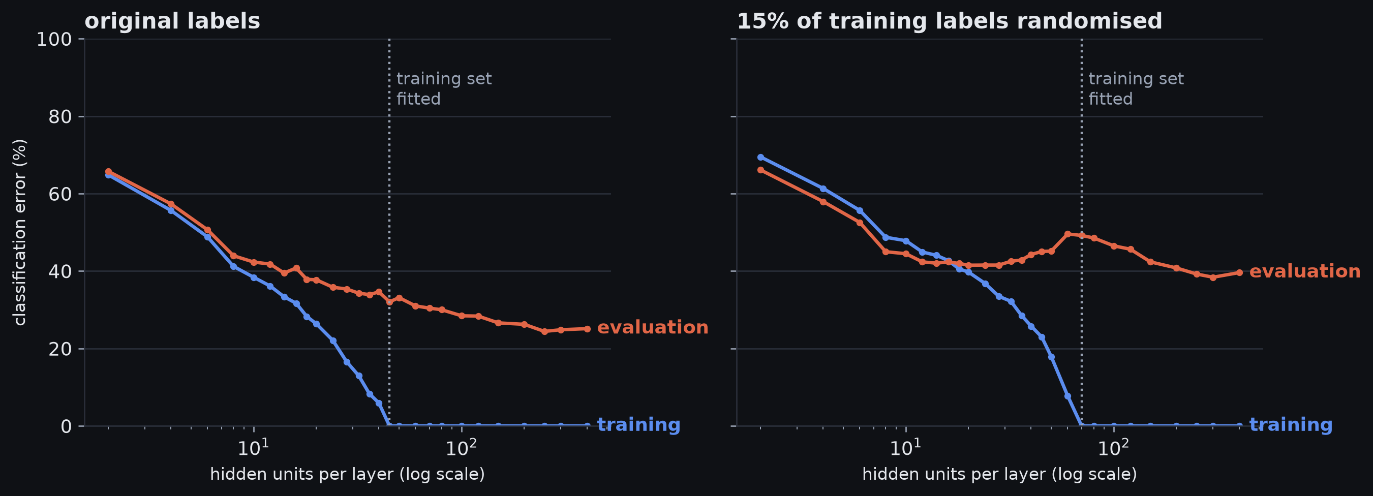
Final training and evaluation error against width, for the original labels (left) and with 15% of the training labels randomised (right); evaluation labels are unchanged in both. The dotted line marks the width at which the training set is first fitted.

Interpolation

A model interpolates a training set when it fits every observed training target exactly under the criterion being discussed.

• in squared-error regression, exact interpolation means passing through every training target and giving zero training squared error
• in classification, zero training classification error is often used as the practical interpolation threshold
• zero classification error does not imply zero cross-entropy: the correct class can be the argmax without having probability one

The interpolation threshold is the effective capacity at which exact fitting first becomes achievable for the training procedure.

Three regimes around interpolation

The curve is commonly divided into three regions:

regime	relationship to fitting the training set
classical / under-parameterised	model cannot yet fit the data exactly
critical	near the point where exact fitting becomes possible
modern / over-parameterised	many parameter settings can fit the training data

The critical point is an effective interpolation threshold; it need not occur exactly when parameter count equals example count.

Interpolating models can still disagree off the training set

Once the training examples are already interpolated:

• once the chosen interpolation criterion is already zero, extra capacity cannot improve that criterion on those observed points
• many distinct functions may agree on every training example
• those functions can behave very differently elsewhere in the input space

Recall: zero classification error is not zero cross-entropy

A classifier can already classify every training example correctly while cross-entropy still decreases as it assigns more probability to the correct classes.

Here, interpolation refers to satisfying the chosen training-fit criterion, not to every possible loss becoming exactly zero.

The remaining question is which compatible solution the learning system tends to reach.

Inductive bias chooses among compatible solutions

Inductive bias is the tendency of a learning system to favour some solutions over others when the observed data do not uniquely determine the function.

It can come from:

• architecture
• parameterisation
• initialisation
• optimiser and optimisation path
• explicit regularisation
• stopping time

Interpolation tells us what happens on the training points; inductive bias helps determine what happens between them.

Why is there so much freedom away from the training set?

Interpolation constrains what the model does on the observed examples. But a finite dataset occupies only a tiny part of a high-dimensional input space.

MNIST-1D already has 40 input dimensions. Suppose, purely for scale, that each dimension were quantised into 10 bins.

The grid would contain

\[ 10^{40} \]

possible cells.

This is a coverage thought experiment, not a claim that real data uniformly occupy all \(10^{40}\) cells. Real datasets can have substantial structure and much lower intrinsic dimension than their raw input dimension.

With \(10^4\) training examples, that is roughly one observed example for every

\[ 10^{36} \]

cells.

This cell count is only a scale argument, but it shows how sparse \(10^4\) observations are relative to even a coarse grid in 40 dimensions.

The curse of dimensionality

At a fixed resolution, the number of regions needed to cover an input space grows exponentially with dimension: \(b\) bins along each of \(D\) dimensions produce \(b^D\) cells.

Consequences include:

• a finite dataset occupies only a tiny fraction of those regions
• keeping the same local sampling density requires rapidly increasing amounts of data
• behaviour away from observed examples becomes increasingly important

The issue is coverage at a chosen resolution, not that every high-dimensional box literally has a larger numerical volume. Low-dimensional diagrams remain useful, but they are only analogies for the geometry of high-dimensional inputs.

Extra capacity permits more interpolating solutions

Sparse observations leave much of the function underconstrained: many functions can agree on every training point while behaving differently elsewhere.

Increasing capacity enlarges the set of functions that can satisfy those observed constraints.

In the low-dimensional illustration, that larger set includes functions that interpolate the same points more smoothly than a near-threshold fit.

Smoothness is therefore one possible compatible behaviour, not a consequence guaranteed by sparsity or capacity. A smoother interpolant can generalise better only when that preference matches the underlying task.

Available does not mean selected: capacity enlarges the set of compatible functions, but does not determine which one training reaches.

Capacity and smooth interpolation

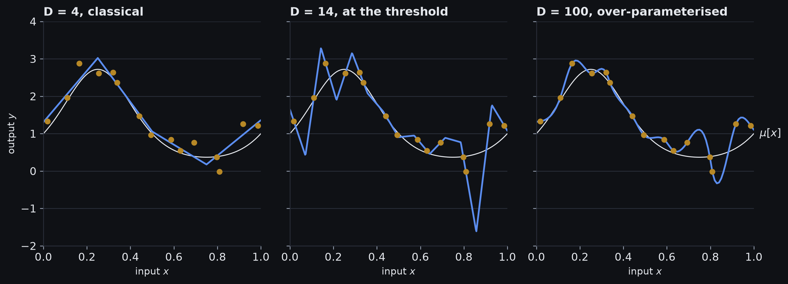
One noisy training set, fitted at three capacities. Left: the classical optimum, which does not pass through the points. Centre: the first capacity that can pass through all of them. Right: far more than enough, with the smallest-norm fit, which is one of many that interpolate.

The training data do not select a unique interpolant

With a heavily over-parameterised model, many functions can fit the same observed training targets exactly or nearly exactly:

• smooth away from the examples
• highly oscillatory away from the examples
• indistinguishable on the observed training targets

The observations constrain the fitted values at the training examples; they do not uniquely specify behaviour elsewhere.

Many zero-loss interpolants

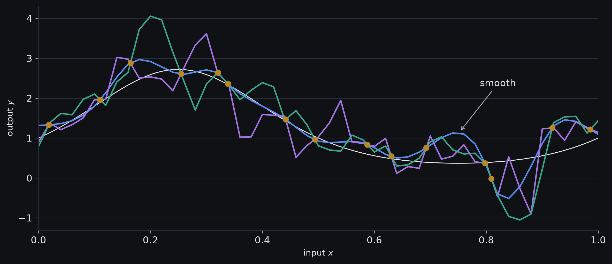
Three over-parameterised models that pass exactly through the same training points, so all three have zero training loss. They differ only in how they behave between the points.

Regularisation as inductive bias

Inductive bias is the broad preference for some compatible solutions over others. Regularisation is one way to create such a preference.

• explicit regularisation deliberately modifies the objective or constraints, for example with weight decay
• implicit regularisation refers to preferences induced by the training dynamics even without an explicit penalty term

Initialisation, optimisation path and stopping time can all affect which interpolating solution is reached. Exactly why particular training systems favour particular solutions is an empirical and theoretical question, not a universal guarantee of smoothness.

Double descent: what it establishes

The experiments establish that evaluation error can improve again after the interpolation threshold.

They do not establish that:

• larger models always generalise better
• interpolation itself guarantees good generalisation
• smoother solutions are automatically selected
• raw parameter count alone determines the regime

The observed curve also depends on dataset and label noise, architecture, loss, optimiser, regularisation and training duration. A related pattern, epoch-wise double descent, can appear when training duration changes while architecture stays fixed.

Advanced qualification: changing dataset size also changes the model’s position relative to the interpolation threshold. In some controlled sweeps, adding examples can therefore move an over-parameterised model back towards the critical regime and temporarily increase evaluation error. This is a qualification to simple monotonic intuitions, not an argument for withholding useful data.

Choosing models without touching the test set

Selection vs assessment

Suppose we train 20 candidate systems. We now need data to answer two different questions:

1. Which system should we choose?
2. How well does the chosen system perform?

If the same held-out results influence the choice and are then reported as untouched evidence, the second answer is no longer independent of the first.

Held-out evaluation vs final test

Earlier, we repeatedly inspected held-out curves to understand training behaviour and double descent.

Once a held-out set influences decisions — even informally — it is part of the development and evaluation loop. It should not also be treated as untouched final evidence for the selected model.

For a final performance estimate, reserve a separate test set until the model, hyperparameters and reporting choices are fixed.

Parameters vs hyperparameters

Parameters \(\params\) are learned inside one training run:

• weights
• biases

Hyperparameters \(\lambda\) configure the model or learning procedure around training runs:

• number of hidden layers
• hidden units per layer
• learning rate
• batch size
• other architectural or optimisation choices

Training chooses \(\params\); model selection chooses \(\lambda\).

The obvious selection method contaminates the test set

A tempting workflow is:

1. train several candidate models
2. score each one on the test set
3. choose the best test score
4. report that same score as final performance

Step 3 uses information from the test set to choose the model. The reported test score is therefore no longer an untouched estimate of performance after selection.

The test set has become part of the model-selection procedure, so it can no longer serve as untouched evidence about the selected system.

Training, validation, and test sets have separate roles

split	used to choose	access pattern
training	model parameters	repeatedly during optimisation
validation	hyperparameters / model choice	repeatedly during development
test	final performance estimate	after development choices are fixed; results must not feed back into selection

The distinction is about information flow, not the filename attached to a dataset.

Hyperparameter selection uses validation performance

For each candidate hyperparameter setting \(\lambda\):

\[ \lambda \longrightarrow \text{train on training set} \longrightarrow \text{validation score}. \]

Choose

\[ \lambda^* = \argmin_{\lambda} \loss_{\mathrm{val}}(\lambda) \]

for a loss metric, or the corresponding \(\arg\max\) for a score.

Reminder: argmin

\(\argmin\) returns the setting \(\lambda\) that gives the smallest validation loss; \(\min\) would return the smallest loss value itself.

Only after \(\lambda^*\) is fixed do we evaluate the selected system on the test set.

Repeated tuning can overfit the validation set too

The validation set is used repeatedly during model selection.

With enough candidate configurations and enough adaptive decisions, some choices can look good partly because they suit quirks of that validation sample.

This is the same generalisation problem at a second level:

• parameters can overfit training data
• hyperparameter decisions can overfit validation data

The untouched test set estimates performance after both levels of selection.

Limited data makes a three-way split expensive

A fixed train/validation/test split with few examples creates tension:

• fewer examples for parameter learning
• fewer examples for reliable validation comparisons
• enough test examples still needed for a useful final estimate

\(K\)-fold cross-validation reuses the training/validation portion more efficiently while keeping the final test set separate.

\(K\)-fold cross-validation rotates the validation fold

Partition the available development data into \(K\) disjoint folds.

For each candidate hyperparameter setting:

1. train on \(K-1\) folds
2. validate on the remaining fold
3. rotate the validation fold through all \(K\) positions
4. average the validation performance

After choosing \(\lambda^*\) from this cross-validation evidence:

1. retrain the selected configuration on all available development data
2. evaluate that fitted system on the untouched final test set

For example, \(K=5\) gives every development example one turn in validation and four turns in training.

Five folds

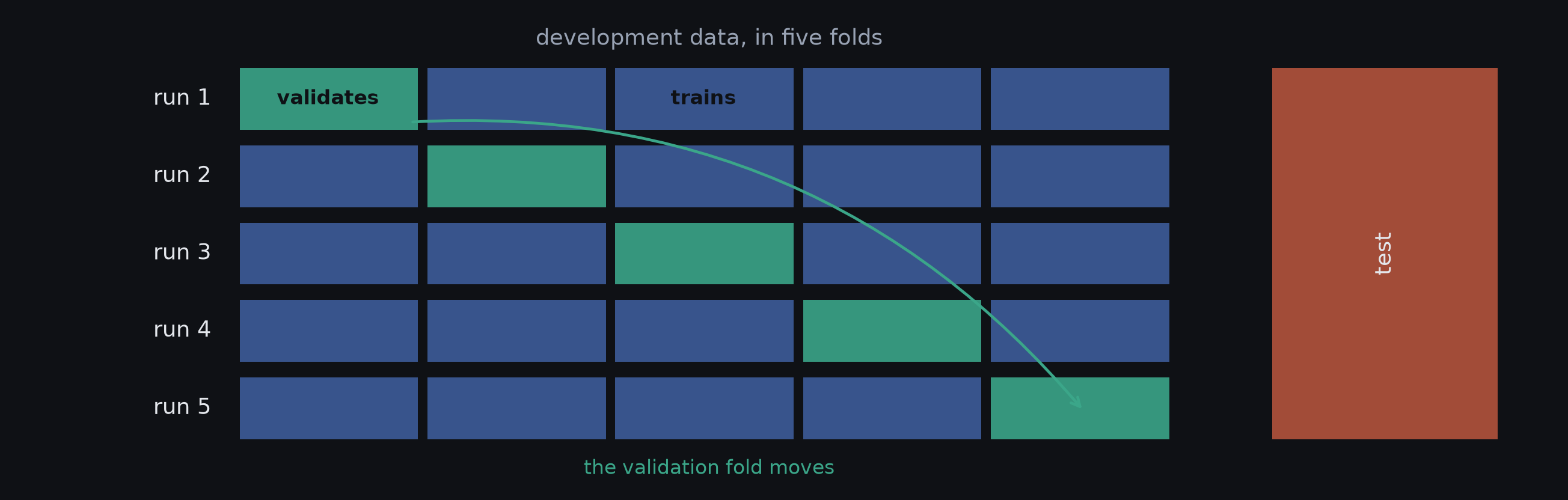
Five-fold cross-validation within the development data. Each row is one training run: four folds train and the fifth validates, and the validation fold moves along. The averaged validation score chooses the hyperparameters; the test set sits apart and is used once, after that choice.

Hyperparameter search

Once validation gives us a way to compare candidate settings, a new problem remains:

Which hyperparameter settings should we spend computation evaluating?

Compared with gradient-based parameter learning, hyperparameter search is awkward because:

• one function evaluation may require a full training run
• many choices are discrete
• some choices are conditional on others
• performance is noisy because training is stochastic
• useful derivatives are generally unavailable

The width of layer 10 is only defined for architectures with at least 10 layers. The search space can therefore contain conditional choices rather than forming one simple rectangular grid.

Hyperparameter search: methods

Three useful families are:

• random search: sample configurations directly
• model-based search: use previous trials to choose promising or informative candidates; Bayesian optimisation is one example
• multi-fidelity search: give many candidates small budgets and allocate more computation to promising runs; Hyperband is one example

The search strategy changes how candidates are explored, not the need for clean validation evidence and a final untouched test set.

Test sets and the deployed world

Test scores and distribution

A test set estimates performance for data distributed like that test set.

If deployment data follow a different distribution, a perfectly untouched test set can still give a misleading estimate of real-world performance.

Evaluation therefore asks two separate questions:

• was the test set kept independent of model selection?
• does the test distribution represent the environment we care about?

Distribution shift can make an old estimate stale

Even a representative test set is a snapshot.

If the deployed data distribution changes over time:

• the old test set becomes less representative
• observed performance can fall
• the model may need monitoring, re-evaluation or retraining

A change in deployment statistics is a form of distribution shift or drift.

One classifier, three ways the world can change

Imagine a vision model that classifies manufactured parts as defective or acceptable.

• covariate shift: the mix or appearance of parts changes, while the same visual evidence still maps to defect status
• label / prior shift: defects become much rarer or more common, while the appearance of defective and acceptable parts within each class remains similar
• concept shift: the production process changes so that old visual cues no longer imply defect status in the same way

These examples are deliberately idealised so that one type of change is isolated at a time.

Three idealised forms of distribution shift

shift	defining change	held stable in the idealised definition
covariate shift	\(p(x)\) changes	\(p(y\mid x)\) remains stable
label / prior shift	\(p(y)\) changes	\(p(x\mid y)\) remains stable
concept shift	\(p(y\mid x)\) changes	no assumption that the old input–output relationship remains valid

Real deployments can contain mixtures of these shifts. The categories are useful because they point to different diagnostics and possible responses.

Scope of a test result

A test result supports a statement of the form:

this selected model achieved this measured performance on this held-out sample from this distribution

After deployment, ask whether:

• the current \(p(x)\) is still represented
• class or target frequencies have changed
• the conditional relationship \(p(y\mid x)\) remains stable
• monitored failures resemble those observed offline

Report the performance number together with the held-out sample and distribution it is intended to represent.

Consolidation

When held-out performance disappoints, ask what changed

Use the ideas from the session as diagnostic questions:

• Does the target vary even at the same observed input? \(\rightarrow\) noise
• Does the average learned function systematically miss the relationship? \(\rightarrow\) bias
• Would a different training sample produce a substantially different model? \(\rightarrow\) variance
• Did this held-out data influence our model choices? \(\rightarrow\) selection contamination
• Does this held-out distribution still represent deployment? \(\rightarrow\) distribution shift

A single performance number cannot answer these questions by itself.

Distinctions to keep separate

• training performance: fit on examples that influenced the parameters
• test performance: performance on held-out examples that did not influence selection
• noise: variation in targets at fixed observed inputs
• bias: systematic deviation of the average fitted predictor from the conditional mean
• variance: sensitivity of the fitted predictor to the sampled training dataset
• overfitting: sample-specific fit that fails to generalise
• capacity: flexibility of the learning system, only imperfectly proxied by parameter count
• regularisation: one source of inductive bias, introduced explicitly through penalties/constraints or implicitly through training dynamics

The least-squares decomposition in one line

At a fixed input \(x\),

\[ \expectsub{\set{D},y}{(\model[{\params[\set{D}]}]{x}-y[x])^2} = \underbrace{ \expectsub{\set{D}}{(\model[{\params[\set{D}]}]{x}-f_\mu[x])^2} }_{\text{variance}} + \underbrace{ (f_\mu[x]-\mu[x])^2 }_{\text{squared bias}} + \underbrace{\sigma^2[x]}_{\text{noise}}. \]

Read it as three questions:

• does the target vary even at the same observed input?
• does the average learned function miss the target mean?
• does the learned function move when the training sample changes?

Classical and over-parameterised regimes

Classical regime

• more capacity can lower bias and raise variance
• expected prediction error may be minimised at intermediate capacity

Over-parameterised regime

• training data may already be interpolated
• many interpolating solutions remain
• inductive biases — including regularisation — influence which one is reached
• held-out error can fall again after the interpolation threshold

Double descent describes the non-monotonic capacity curve in which held-out error can fall again beyond the interpolation threshold.

Data splits

• training set chooses parameters
• validation evidence chooses hyperparameters and model variants
• test set estimates performance after those choices are fixed
• \(K\)-fold cross-validation can use limited pre-test data more efficiently
• repeated selection against the test set destroys its role as an untouched final estimate

The test set is protected because we want one sample that did not participate in deciding what system to report.

Performance after deployment can still change

An untouched test estimate can become stale when the deployment distribution changes.

• covariate shift changes \(p(x)\) while \(p(y\mid x)\) remains stable in the idealised case
• label / prior shift changes \(p(y)\) while \(p(x\mid y)\) remains stable in the idealised case
• concept shift changes \(p(y\mid x)\)
• distribution shift can make a once-representative test set stale

A deployed model therefore needs both initial evaluation and ongoing monitoring.

Source and revision locators

• Simon J. D. Prince, Understanding Deep Learning, Chapter 8: “Measuring performance” (Prince 2023)
• MNIST background: Yann LeCun, Corinna Cortes and Christopher J. C. Burges, The MNIST Database of Handwritten Digits
• MNIST-1D construction and motivation: Sam Greydanus and Dmitry Kobak, Scaling Down Deep Learning with MNIST-1D (ICML 2024)
• Sections: 8.1 training a simple model; 8.2 sources of error; 8.3 reducing error; 8.4 double descent; 8.5 choosing hyperparameters; 8.6 summary
• Core derivation: equations 8.1–8.7
• Notebooks: 8.1 MNIST-1D performance; 8.2 bias–variance trade-off; 8.3 double descent; 8.4 high-dimensional spaces
• Chapter notes used here: cross-validation, capacity, double descent, curse of dimensionality, real-world performance, hyperparameter search
• Problems: 8.1–8.9 for derivation and high-dimensional-space practice

Prince, Simon J. D. 2023. Understanding Deep Learning. MIT Press. https://udlbook.github.io/udlbook/.