Lecture 5: Gradients and Initialisation

Block 4.2 Advanced AI

Eoin O’Brien

Gradients in deep networks

Gradient computation

• a neural network maps inputs to predictions through many composed calculations
• a loss maps those predictions to one scalar
• an optimiser changes the parameters using the gradient of that scalar loss
• training therefore needs a derivative with respect to every parameter

Computing every parameter derivative independently would repeat the same downstream chain-rule calculations thousands or millions of times.

Learning goals

By the end of this lecture, you should be able to:

• explain why naive gradient calculations repeat work
• explain the forward and backward passes in backpropagation
• derive backpropagation first for scalar calculations, then for vector-valued layers
• read the matrix expressions for bias, weight, and activation gradients
• explain why neural-network training uses reverse-mode differentiation
• derive the scaling logic behind Kaiming/He initialisation for ReLU networks
• connect the mathematical derivation to a complete training loop

Two neural-network-specific problems

Training requires repeated gradient-based updates. For neural networks, two practical questions dominate:

1. Gradient computation: how do we obtain derivatives with respect to every weight and bias without duplicating work?

2. Initialisation: how do we choose starting weights so that activations and gradients remain numerically well-scaled through many layers?

• keep the two questions distinct: backpropagation is about efficient derivative computation; initialisation is about the scale of forward and backward signals

Weights and biases

For trainable model parameters, we follow Prince’s Greek-letter notation:

• \(\params\) — all trainable parameters collected together
• \(\layerweights_k\) — the weight matrix of layer \(k\)
• \(\layerbias_k\) — the bias vector of layer \(k\)

The familiar affine map

\[ \mat{W}\vect{x}+\vect{b} \]

is written in Prince, Chapter 7, as (Prince 2023)

\[ \vect{f}_k = \layerbias_k+\layerweights_k\hidden_k. \]

The arithmetic is unchanged; the Greek symbols make the learned quantities explicit.

• this is a reminder, not a new convention – the seam was taught in week 1
• students will read both this week: Chapter 7 in Greek notation, PyTorch in .weight and .bias

Why those letters

The letters are chosen to be memorable:

• \(\layerweights_k\): capital omega, and lowercase \(\omega\) is the letter drawn like a w, for weights
• \(\layerbias_k\): beta, the Greek b, for bias
• \(\hidden_k\): the layer’s hidden activations, the \(\vect{x}\) that this layer happens to see
• \(\vect{f}_k\): the pre-activation, before the nonlinearity makes \(\hidden_{k+1}\)

Shapes and orientation

For a layer taking \(\dimension_k\) activations to \(\dimension_{k+1}\):

object	shape
\(\hidden_k\)	\(\dimension_k\times1\)
\(\layerweights_k\)	\(\dimension_{k+1}\times\dimension_k\)
\(\layerbias_k\)	\(\dimension_{k+1}\times1\)
\(\vect{f}_k\)	\(\dimension_{k+1}\times1\)

The weight matrix is read right to left: it takes \(\dimension_k\) numbers in and gives \(\dimension_{k+1}\) out.

Layer indexing

For affine layer \(k\):

• \(\hidden_k\) — the source activations entering the layer
• \(\vect{f}_k\) — the destination pre-activations produced by the layer
• \(\hidden_{k+1}=\vactivation{\vect{f}_k}\) — the next activations after the nonlinearity

The repeated pattern is

\[ \hidden_k \longrightarrow \vect{f}_k \longrightarrow \hidden_{k+1}. \]

Network anatomy

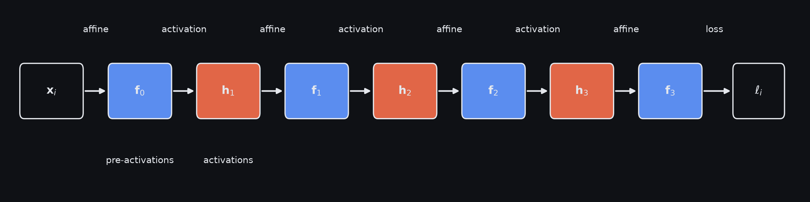
A deep network alternates affine maps and elementwise nonlinearities. The loss is attached only at the end, but every earlier parameter influences it through the chain of computations.

A three-hidden-layer network

For one training example \(\vect{x}_i\):

\[ \begin{aligned} \vect{f}_0 &= \layerbias_0+\layerweights_0\vect{x}_i \\ \hidden_1 &= \vactivation{\vect{f}_0} \\ \vect{f}_1 &= \layerbias_1+\layerweights_1\hidden_1 \\ \hidden_2 &= \vactivation{\vect{f}_1} \\ \vect{f}_2 &= \layerbias_2+\layerweights_2\hidden_2 \\ \hidden_3 &= \vactivation{\vect{f}_2} \\ \vect{f}_3 &= \layerbias_3+\layerweights_3\hidden_3 \end{aligned} \]

The per-example loss is

\[ \exloss_i = \exloss(\vect{f}_3,\vect{y}_i). \]

The gradient required by SGD

Chapter 7 writes the full training loss as a sum:

\[ \loss[\params] = \sum_{i=1}^{I}\exloss_i. \]

For a batch \(\mathcal B_t\), the SGD update is

\[ \params_{t+1} = \params_t - \alpha \sum_{i\in\mathcal B_t} \nabla_{\params}\exloss_i. \]

Every update therefore needs the derivative of one scalar loss with respect to a very large collection of parameters.

Candidate 1: perturb every parameter

A programmer’s first idea might be numerical differentiation:

\[ \frac{\partial\exloss}{\partial\phi_j} \approx \frac{ \exloss(\params+\varepsilon\vect{e}_j) - \exloss(\params-\varepsilon\vect{e}_j) }{2\varepsilon}. \]

Here \(\vect{e}_j\) is zero everywhere except position \(j\), so only parameter \(\phi_j\) is perturbed.

For \(P\) parameters, centred finite differences require roughly \(2P\) forward evaluations to recover the full gradient.

• 8 parameters in our scalar toy model → about 16 evaluations
• \(10^6\) parameters → about 2 million evaluations

Finite differences are valuable for checking a gradient, not for computing every training update.

Candidate 2: differentiate each parameter separately

The chain rule can give an exact derivative for any one parameter. For an early scalar weight,

\[ \frac{\partial\exloss_i}{\partial\omega_0} = \frac{\partial f_0}{\partial\omega_0} \frac{\partial h_1}{\partial f_0} \frac{\partial f_1}{\partial h_1} \cdots \frac{\partial\exloss_i}{\partial f_3}. \]

For \(\omega_1\), much of the right-hand side is the same downstream chain again. For \(\omega_2\), it appears again.

The derivatives are exact, but calculating each one independently repeats work.

Shared downstream paths

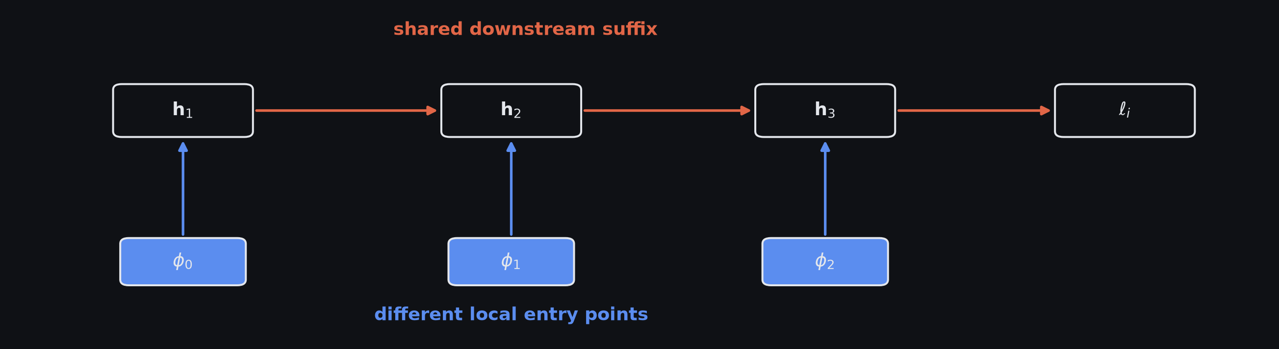
Parameters at different depths have different path lengths to the loss, but the right-hand suffixes of those paths are shared. Computing every derivative independently would repeatedly rebuild those same suffixes.

Repeated derivative work

Computing each parameter derivative separately rebuilds the same downstream derivative products.

Compute each shared downstream sensitivity once, cache it, and reuse it.

Candidate 3: reuse what repeats

Start at the only quantity we ultimately care about: the loss. Then repeatedly ask one local question:

if this intermediate value changed a little, how much would the loss change?

Each answer becomes an input to the next question one step earlier in the graph.

• compute values forward
• compute loss sensitivities backward
• reuse each sensitivity instead of rebuilding the full chain

Why propagate derivatives backward?

A neural network has many parameters but one scalar loss:

\[ \exloss:\mathbb{R}^{P}\rightarrow\mathbb{R}. \]

Two derivative-propagation strategies have very different pass counts for the full gradient. Here a seed is the derivative value propagation starts from; reverse mode starts at the loss with \(\partial\exloss/\partial\exloss=1\).

mode	seed	sweeps for all \(P\) partial derivatives
forward mode	one parameter direction	\(P\)
reverse mode	the scalar loss	\(1\)

For the eight-parameter toy model: 8 forward-mode seeds versus 1 reverse seed. For \(P=10^6\): the pass-count asymmetry is \(10^6\) versus \(1\).

Each sweep still traverses the computation graph; the advantage is the number of sweeps.

One seed, or one seed per parameter

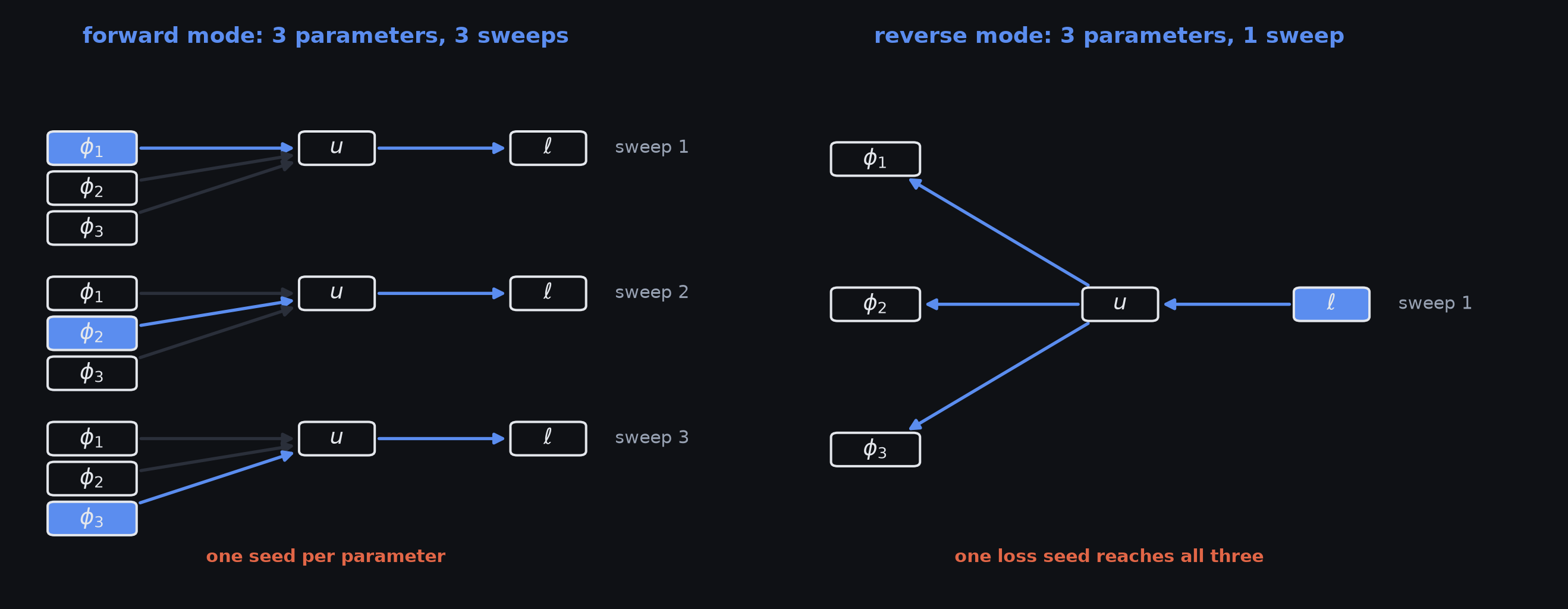
Forward mode seeds one parameter direction and moves toward the loss, so three parameters require three sweeps. Reverse mode seeds the one scalar loss and reaches all three parameters in one reverse sweep.

• the asymmetry comes from the problem shape: many inputs to the derivative calculation, one scalar output
• the three copies on the left are separate derivative sweeps, not network layers
• do not claim a reverse sweep is constant-time; it still traverses the graph

Forward and backward passes

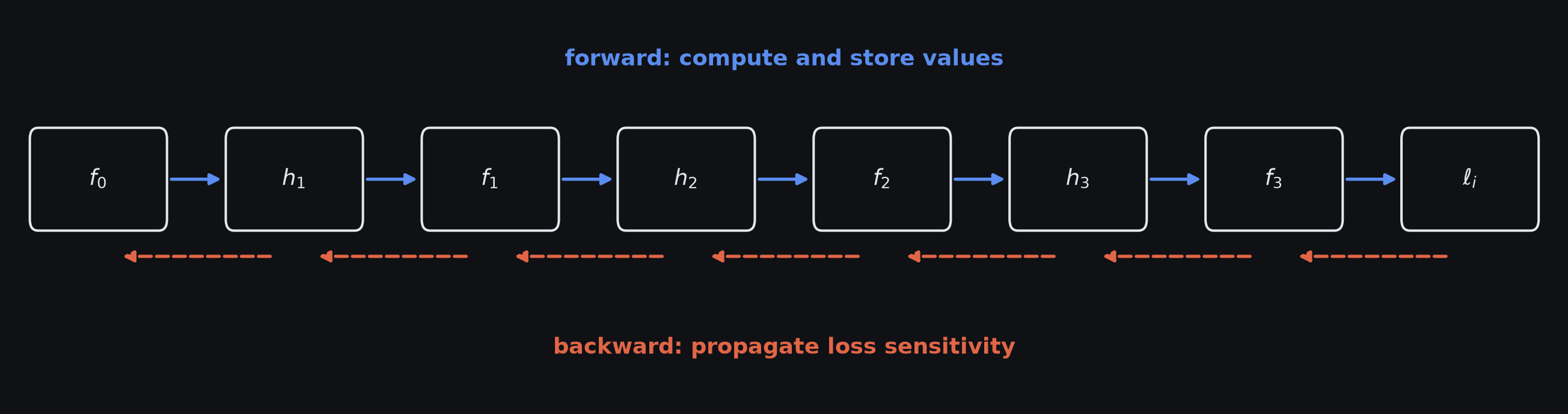
The forward pass stores intermediate values. The backward pass propagates one cached loss sensitivity at a time in the opposite direction.

Why the forward values are kept

The backward pass needs two kinds of stored forward value:

• an activation derivative needs the stored pre-activation
• a weight gradient needs the stored activation entering that weight

Reusing derivative work therefore requires memory for these forward intermediates.

Backpropagation in scalars

Scalar running example

Use the one-unit-per-layer toy model from Section 7.3:

\[ \begin{aligned} f_0 &= \beta_0+\omega_0x_i \\ h_1 &= \sin(f_0) \\ f_1 &= \beta_1+\omega_1h_1 \\ h_2 &= \exp(f_1) \\ f_2 &= \beta_2+\omega_2h_2 \\ h_3 &= \cos(f_2) \\ f_3 &= \beta_3+\omega_3h_3 \\ \exloss_i &= (f_3-y_i)^2 \end{aligned} \]

The deliberately different \(\sin\), \(\exp\), and \(\cos\) operations are not a proposed network architecture. They force us to apply the chain rule through several different local functions instead of memorising one derivative.

The computation graph

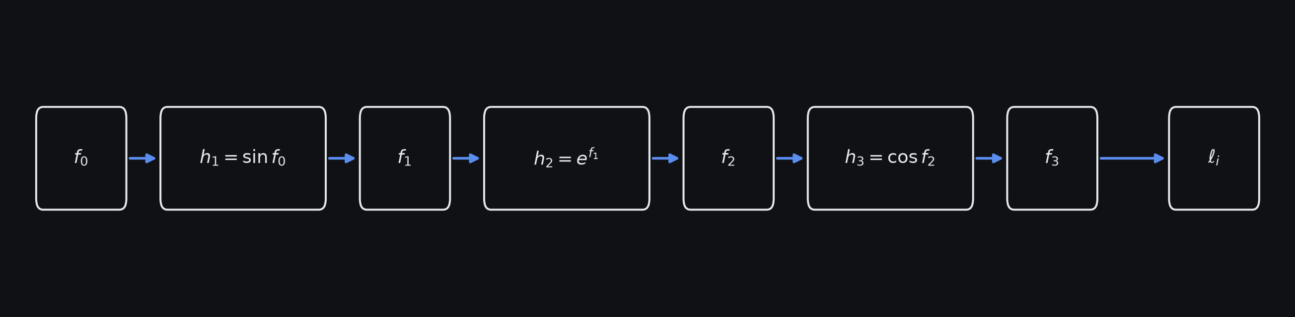
Breaking the composed expression into named intermediate values exposes the local calculations that the chain rule will reuse.

The forward pass numerically

Take

\[ x_i=0.5,\qquad y_i=0.2 \]

and

\[ \begin{aligned} \layerbias &= [0.1,\,-0.2,\,0.05,\,0.15]\transpose \\ \vect{\omega} &= [0.8,\,1.1,\,-0.7,\,0.9]\transpose. \end{aligned} \]

The forward pass gives approximately

quantity	value
\(f_0\)	0.500
\(h_1\)	0.479
\(f_1\)	0.327
\(h_2\)	1.387
\(f_2\)	-0.921
\(h_3\)	0.605
\(f_3\)	0.694
\(\exloss_i\)	0.244

Chain rule refresher

If

\[ u=g(v), \qquad L=q(u), \]

then a small change in \(v\) first changes \(u\), which then changes \(L\).

The local sensitivities multiply:

\[ \frac{dL}{dv} = \frac{du}{dv} \frac{dL}{du}. \]

Read right-to-left:

how much does \(u\) change with \(v\) × how much does \(L\) change with \(u\)?

Loss sensitivity: the cached quantity

For every pre-activation, define

\[ \delta_k \equiv \frac{\partial\exloss_i}{\partial f_k}. \]

Read \(\delta_k\) as:

how much does the loss currently care about a small change in \(f_k\)?

• the sign tells whether increasing \(f_k\) would locally increase or decrease the loss
• the magnitude tells how strongly the loss responds locally
• most importantly, once \(\delta_k\) has been computed, earlier layers can reuse it

Seed the backward pass at the loss

The final operation is

\[ \exloss_i=(f_3-y_i)^2. \]

Therefore

\[ \boxed{ \delta_3 = \frac{\partial\exloss_i}{\partial f_3} = 2(f_3-y_i) } \]

For the numerical example,

\[ \delta_3\approx 0.989. \]

This is the one derivative we can compute immediately from the loss.

One step backward

First pass sensitivity through the affine operation

\[ f_3=\beta_3+\omega_3h_3. \]

Since \(\partial f_3/\partial h_3=\omega_3\),

\[ \frac{\partial\exloss_i}{\partial h_3} = \omega_3\delta_3. \]

Then pass it through

\[ h_3=\cos(f_2), \]

so

\[ \boxed{ \delta_2 = -\sin(f_2)\,\omega_3\,\delta_3. } \]

One backward step is therefore

\[ \text{downstream sensitivity} \times \text{local linear effect} \times \text{local activation derivative}. \]

Repeat the same local recipe

The next two steps use exactly the same pattern:

\[ \delta_1 = \exp(f_1)\,\omega_2\,\delta_2 \]

and

\[ \delta_0 = \cos(f_0)\,\omega_1\,\delta_1. \]

In general,

\[ \boxed{ \delta_{k-1} = \dactivation{f_{k-1}}\,\omega_k\,\delta_k. } \]

The long chain-rule expression is never rebuilt from scratch.

Forward values and backward sensitivities

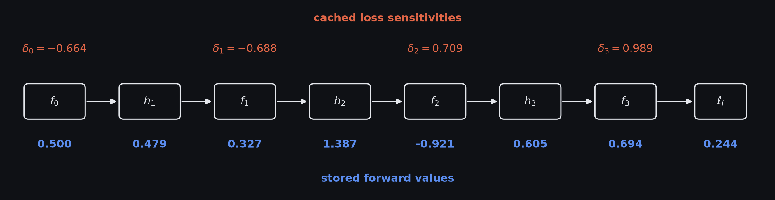
The forward pass stores numerical values at every intermediate quantity. The backward pass attaches one cached loss sensitivity \(\delta_k\) to each pre-activation.

The chain of multipliers

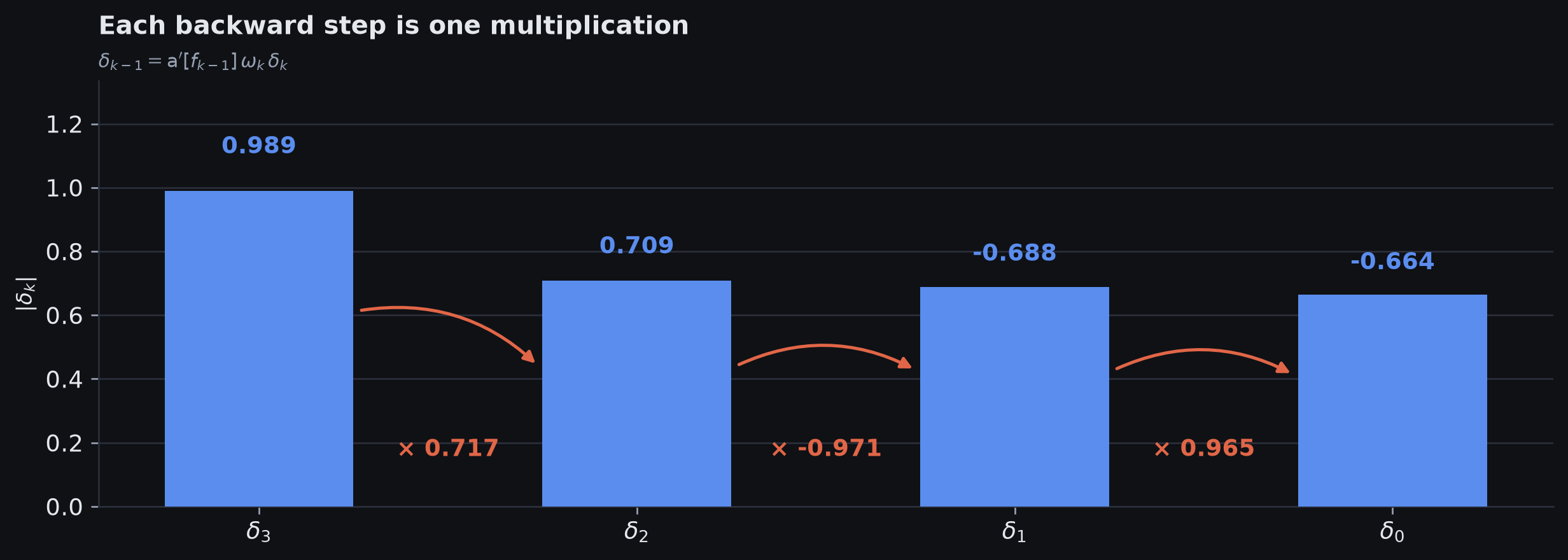
Each cached scalar sensitivity is obtained from the one to its right by multiplying by one local factor. Repeating factors systematically above or below one can grow or shrink sensitivities through depth.

• read it right to left, which is the direction the pass runs
• hold this picture for initialisation: repeated local multipliers can shrink or grow a signal through depth

Parameter gradients reuse the same sensitivity

Once \(\delta_k\) is known, the parameters feeding into \(f_k\) use the same cached sensitivity. For \(k>0\),

\[ f_k=\beta_k+\omega_kh_k. \]

Therefore

\[ \boxed{ \frac{\partial\exloss_i}{\partial\beta_k}=\delta_k, \qquad \frac{\partial\exloss_i}{\partial\omega_k}=h_k\delta_k. } \]

For the first layer, replace the source activation \(h_0\) by the input \(x_i\):

\[ \frac{\partial\exloss_i}{\partial\omega_0}=x_i\delta_0. \]

The gradient of a weight is signal through the connection × loss sensitivity at its destination.

Finite differences return as a check

We rejected finite differences as the training algorithm because they require roughly \(2P\) forward evaluations. They are still useful for checking one analytic or automatic derivative:

\[ \frac{\partial\exloss_i}{\partial\omega_0} \approx \frac{ \exloss_i(\omega_0+\varepsilon) - \exloss_i(\omega_0-\varepsilon) }{2\varepsilon}. \]

With \(\varepsilon=10^{-5}\):

• Backpropagation: -0.3321784044
• Finite difference: -0.3321784044

• explicitly call back to Candidate 1: rejected for scale, retained as a debugging check

Scalar backpropagation

The scalar algorithm is now:

1. run the model forward and store intermediate values
2. seed the loss sensitivity at the final output
3. propagate one cached sensitivity backward through each local operation
4. reuse that sensitivity to form the local parameter gradients
5. continue toward the input

Backpropagation stores local forward values and cached local sensitivities instead of expanding one full symbolic derivative.

Vector and matrix backpropagation

One scalar sensitivity becomes one per unit

The scalar equation

\[ f_k=\beta_k+\omega_kh_k \]

becomes

\[ \vect{f}_k = \layerbias_k + \layerweights_k\hidden_k. \]

A layer has several destination pre-activations \(\vect{f}_k\), so it has one loss sensitivity for each destination unit. The source activations \(\hidden_k\) are the values entering the affine layer; the resulting \(\vect{f}_k\) are its pre-activations. Stack the destination sensitivities into a column:

\[ \sensitivity_k \equiv \nabla_{\vect{f}_k}\exloss_i. \]

The same loss-sensitivity idea now has one component per unit. The new feature is that several downstream paths can contribute to one earlier unit.

A small vector-valued layer

Take a layer with two source activations and three destination pre-activations:

Two sources, three destinations

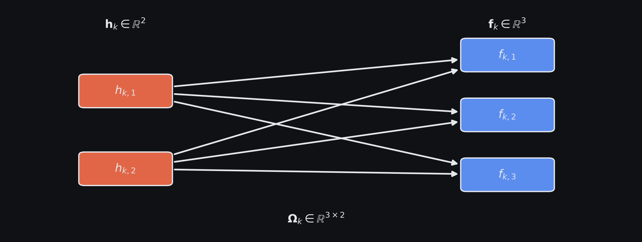
A small 2→3 affine layer. We will derive the backward rules by asking what each source activation and each weight contributes to the loss.

Shapes in this example

For this example,

\[ \hidden_k:2\times1, \qquad \layerweights_k:3\times2, \qquad \vect{f}_k,\layerbias_k,\sensitivity_k:3\times1. \]

Gather sensitivity back to one source

Suppose the destination sensitivities are

\[ \sensitivity_k = \begin{bmatrix} \delta_{k,1}\\ \delta_{k,2}\\ \delta_{k,3} \end{bmatrix}. \]

Changing source activation \(h_{k,1}\) changes all three destination pre-activations. Therefore all three paths contribute:

\[ \boxed{ \frac{\partial\exloss_i}{\partial h_{k,1}} = \Omega_{k,11}\delta_{k,1} + \Omega_{k,21}\delta_{k,2} + \Omega_{k,31}\delta_{k,3}. } \]

This is just the chain rule adding the contributions from every path out of \(h_{k,1}\).

Do both source activations at once

The second source activation similarly gives

\[ \frac{\partial\exloss_i}{\partial h_{k,2}} = \Omega_{k,12}\delta_{k,1} + \Omega_{k,22}\delta_{k,2} + \Omega_{k,32}\delta_{k,3}. \]

Stack the two answers:

\[ \begin{bmatrix} \partial\exloss_i/\partial h_{k,1}\\ \partial\exloss_i/\partial h_{k,2} \end{bmatrix} = \begin{bmatrix} \Omega_{k,11}&\Omega_{k,21}&\Omega_{k,31}\\ \Omega_{k,12}&\Omega_{k,22}&\Omega_{k,32} \end{bmatrix} \sensitivity_k. \]

The matrix on the right is exactly \(\layerweights_k\transpose\):

\[ \boxed{ \nabla_{\hidden_k}\exloss_i = \layerweights_k\transpose\sensitivity_k. } \]

Why the transpose appears

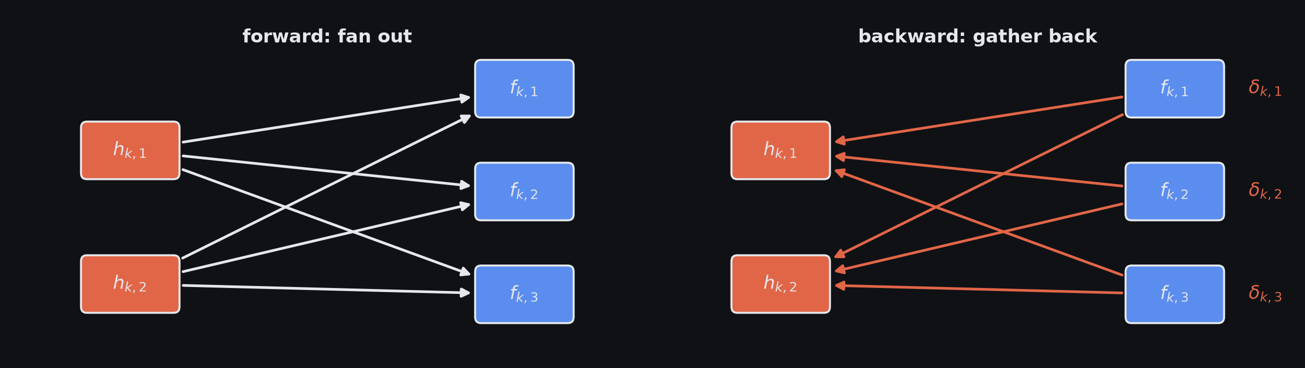
Forward, one source activation fans out through a column of the weight matrix. Backward, the loss contributions on those same connections are gathered back to that source. Doing the gathering for every source at once is multiplication by the transpose.

Formal check with first-order changes

For a scalar loss and vector \(\vect{z}\), the gradient dotted with a proposed small change \(\Delta\vect{z}\) predicts the corresponding first-order change in the loss. With column-vector gradients:

\[ \Delta\exloss_i \approx \left(\nabla_{\vect{z}}\exloss_i\right)\transpose\Delta\vect{z}. \]

For the affine layer,

\[ \Delta\vect{f}_k = \layerweights_k\Delta\hidden_k, \]

so

\[ \Delta\exloss_i \approx \sensitivity_k\transpose\layerweights_k\Delta\hidden_k = \left(\layerweights_k\transpose\sensitivity_k\right)\transpose\Delta\hidden_k. \]

This must agree with

\[ \Delta\exloss_i \approx \left(\nabla_{\hidden_k}\exloss_i\right)\transpose\Delta\hidden_k \]

for every \(\Delta\hidden_k\). Therefore the coefficient vectors are equal:

\[ \nabla_{\hidden_k}\exloss_i = \layerweights_k\transpose\sensitivity_k. \]

ReLU is a gate on the backward pass

Suppose a ReLU layer saw

\[ \vect{f}_{k-1} = \begin{bmatrix} -1.2\\ 0.4\\ 2.1 \end{bmatrix} \]

and the sensitivity arriving at its activation vector is

\[ \nabla_{\hidden_k}\exloss_i = \begin{bmatrix} 3\\ -2\\ 5 \end{bmatrix}. \]

The first ReLU was off in the forward pass, so it blocks the backward signal. The other two were on, so they pass it through:

\[ \boxed{ \sensitivity_{k-1} = \begin{bmatrix} 0\\ -2\\ 5 \end{bmatrix}. } \]

For ReLU, backpropagation through the activation is simply a stored on/off mask from the forward pass.

The formal ReLU rule

For

\[ \relu(z)=\max(0,z), \]

away from \(z=0\),

\[ \relu'(z) = \begin{cases} 0,&z<0\\ 1,&z>0. \end{cases} \]

Applied elementwise, \(\indicator{\text{condition}}\) is \(1\) where the condition is true and \(0\) otherwise, and \(\odot\) means component-by-component multiplication:

\[ \boxed{ \sensitivity_{k-1} = \indicator{\vect{f}_{k-1}>0} \odot \left( \layerweights_k\transpose\sensitivity_k \right). } \]

Formally, the Jacobian of an elementwise activation is diagonal: each ReLU output depends only on the matching input, so all cross-unit partial derivatives are zero. For ReLU, the diagonal is exactly the \(0/1\) mask above.

One weight first

Consider the weight \(\Omega_{k,rc}\) connecting source activation \(h_{k,c}\) to destination pre-activation \(f_{k,r}\).

A small weight change produces

\[ \Delta f_{k,r} = h_{k,c}\,\Delta\Omega_{k,rc}. \]

The loss sensitivity at that destination is \(\delta_{k,r}\), so

\[ \boxed{ \frac{\partial\exloss_i}{\partial\Omega_{k,rc}} = \delta_{k,r}h_{k,c}. } \]

Every weight needs exactly two local numbers:

• source activation: how much signal travelled through the connection
• destination sensitivity: how much the loss cares about where the connection lands

Fill the whole weight-gradient matrix

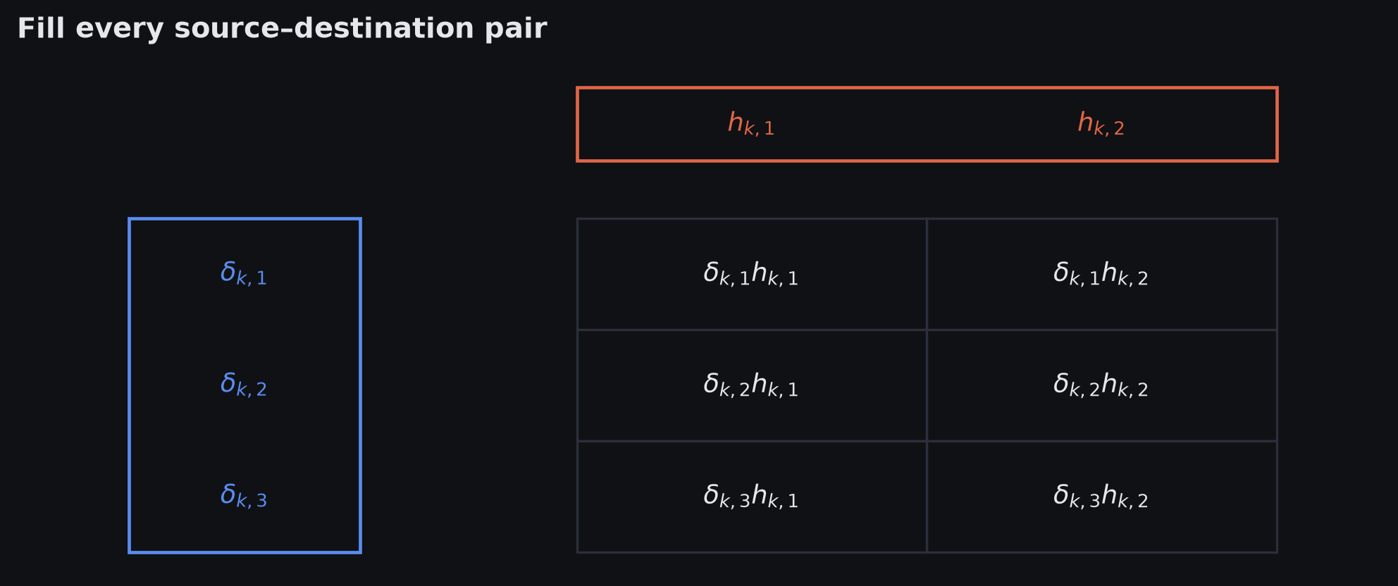
Each cell of the weight-gradient matrix is one destination sensitivity times one source activation. Filling every source–destination pair produces the outer product.

The outer product

Linear algebra has a name for exactly this construction: an outer product. A dot product combines two vectors into one number; an outer product forms the matrix of all pairwise products.

\[ \boxed{ \nabla_{\layerweights_k}\exloss_i = \sensitivity_k\hidden_k\transpose. } \]

The shape is automatically the shape of the weight matrix:

\[ (\dimension_{k+1}\times1)(1\times\dimension_k) = \dimension_{k+1}\times\dimension_k. \]

Bias gradients are simpler

Because adding the bias changes the corresponding pre-activation one-for-one,

\[ \Delta\vect{f}_k = \Delta\layerbias_k. \]

Therefore

\[ \boxed{ \nabla_{\layerbias_k}\exloss_i = \sensitivity_k. } \]

The sensitivity already stored at the layer is its bias gradient.

One layer viewed backward

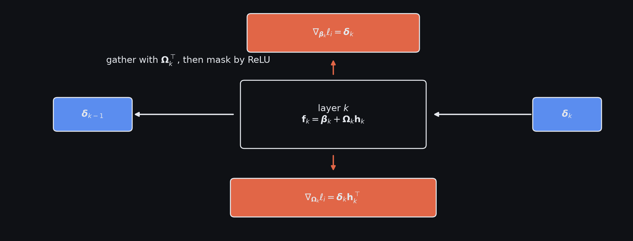
One backward traversal of an affine-plus-ReLU layer does three jobs: form the bias gradient, form the weight gradient, and pass a masked sensitivity to the previous layer.

Backpropagation recurrence

For a ReLU network,

\[ \boxed{ \begin{aligned} \nabla_{\layerbias_k}\exloss_i &= \sensitivity_k \\ \nabla_{\layerweights_k}\exloss_i &= \sensitivity_k\hidden_k\transpose \\ \sensitivity_{k-1} &= \indicator{\vect{f}_{k-1}>0} \odot \left( \layerweights_k\transpose\sensitivity_k \right) \end{aligned} } \]

Chapter 7, equation 7.25 (Prince 2023)

Read the three lines as:

1. bias: use the destination sensitivity directly
2. weights: pair each destination sensitivity with each source activation
3. previous layer: gather sensitivity through the same connections, then apply the activation gate

The first layer

The first pre-activation uses the input rather than a hidden activation:

\[ \vect{f}_0 = \layerbias_0 + \layerweights_0\vect{x}_i. \]

Once \(\sensitivity_0\) is available,

\[ \boxed{ \nabla_{\layerbias_0}\exloss_i = \sensitivity_0, \qquad \nabla_{\layerweights_0}\exloss_i = \sensitivity_0\vect{x}_i\transpose. } \]

Backpropagation algorithm

Forward pass

• compute each pre-activation and activation
• compute the prediction and scalar loss
• store the local values required later

Backward pass

1. seed the loss sensitivity at the output
2. form that layer’s bias and weight gradients
3. gather sensitivity through the transposed weights
4. apply the activation derivative or mask
5. repeat toward the input

This is the vector form of exactly the scalar algorithm we already ran by hand.

Batch gradients

Backpropagation above computes gradients for one training example. Under the sum convention used here,

\[ \nabla_{\params} \sum_{i\in\mathcal B_t}\exloss_i = \sum_{i\in\mathcal B_t} \nabla_{\params}\exloss_i. \]

A batch mean instead divides that sum by \(|\mathcal B_t|\). The local backpropagation rules do not change; only the reduction across examples changes the final scale.

Compute versus memory

The expensive operations in both passes are matrix multiplications:

• forward — \(\layerweights_k\hidden_k\)
• backward — \(\layerweights_k\transpose\sensitivity_k\)

Backpropagation avoids repeated chain-rule work by reusing cached sensitivities. The price is memory: the backward pass still needs values saved during the forward pass.

This is the same trade-off we saw at the start:

compute once, store, reuse rather than recompute the same derivative suffix repeatedly.

Algorithmic differentiation

Reverse-mode algorithmic differentiation

Backpropagation is reverse-mode algorithmic differentiation applied to a neural-network computation graph.

A framework does not need one giant hand-written derivative for the model. Each primitive operation needs only:

• its forward computation
• the local rule for sending sensitivity to its inputs
• the local rule for its parameters, if it has any

The scalar and vector derivations above are those local rules written out by hand.

Branching graphs

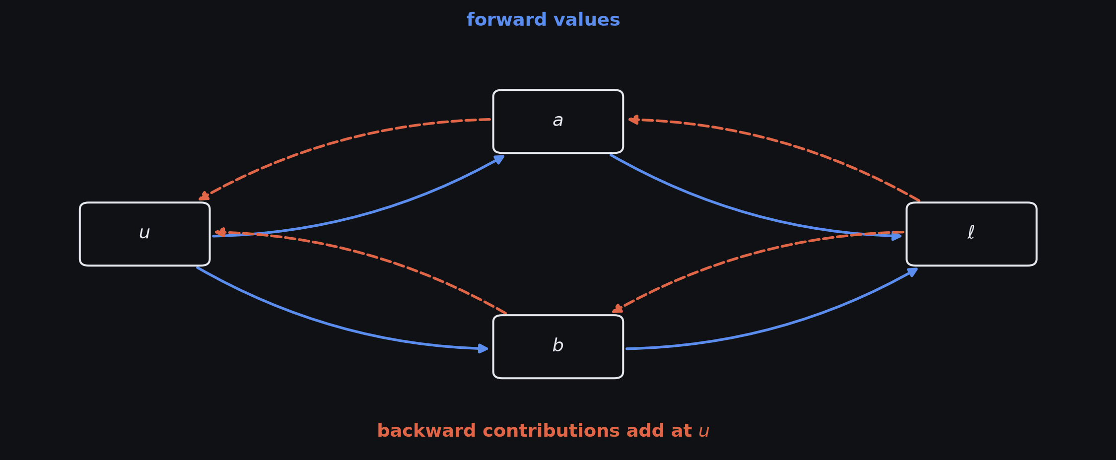
Backpropagation is not restricted to a chain. When one quantity influences the loss through several branches, reverse mode adds the sensitivity contributions from every downstream path.

Adding contributions at a shared ancestor

If

\[ u\to a\to\exloss \qquad\text{and}\qquad u\to b\to\exloss, \]

then

\[ \frac{d\exloss}{du} = \frac{\partial a}{\partial u}\frac{\partial\exloss}{\partial a} + \frac{\partial b}{\partial u}\frac{\partial\exloss}{\partial b}. \]

Reverse mode accumulates those contributions at the shared ancestor.

Tensors and batches

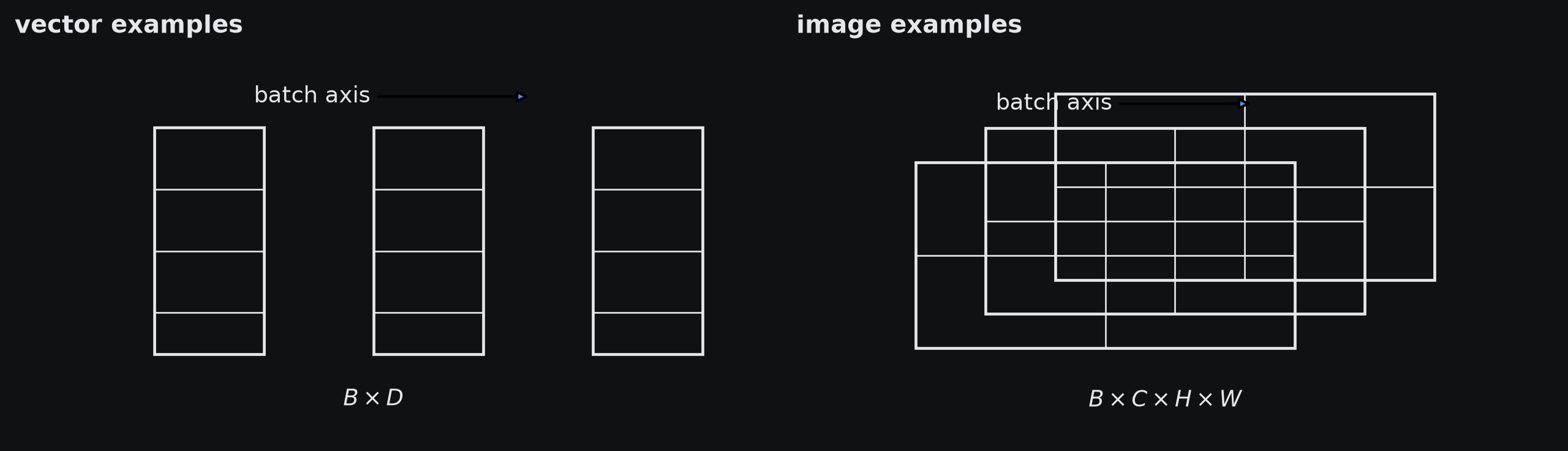
Batching adds one extra axis. A batch is a stack of examples of the same underlying object; the local derivative rules are applied across that additional axis.

Batch shapes

• vector example — \(\dimension\) becomes batch shape \(B\times\dimension\)
• RGB image — \(H\times W\times C\) becomes \(B\times C\times H\times W\)

The derivative rules are unchanged; batching adds an axis over examples.

One training iteration

In PyTorch-style pseudocode:

optimizer.zero_grad()
prediction = model(x_batch)
loss = criterion(prediction, y_batch)
loss.backward()
optimizer.step()

• model(...) — run the forward graph and save required intermediates
• loss.backward() — seed the scalar loss and run reverse-mode accumulation
• optimizer.step() — update parameters using the accumulated gradients

Inside loss.backward()

The framework is automating the operations we have already derived:

• traverse the computation graph in reverse
• gather sensitivities with transposed weight matrices
• apply activation derivative masks
• form weight gradients from destination sensitivity × source activation
• add contributions where graph paths meet
• reduce contributions across the batch according to the loss convention

loss.backward() applies these local derivative rules while traversing the computation graph in reverse.

Parameter initialisation

Parameters need a starting point

Before the first training update, every weight and bias already needs a value.

Why not initialise everything to zero and let gradient descent take it from there?

Zero initialisation makes all hidden units start identically.

Candidate 1: initialise every weight to zero

Suppose two hidden units have identical incoming weights and biases.

For every input,

\[ f_a=f_b \qquad\Longrightarrow\qquad h_a=h_b. \]

If the surrounding network is symmetric as well, backpropagation gives

\[ \delta_a=\delta_b. \]

Their incoming-weight gradients are therefore identical:

\[ \nabla_{\vect{\omega}_a}\exloss = \delta_a\hidden\transpose = \delta_b\hidden\transpose = \nabla_{\vect{\omega}_b}\exloss. \]

They take the same update and remain identical.

• zero is the cleanest student proposal, but the deeper failure is identical initialisation, not the particular number zero
• with ReLU, all-zero weights create additional trouble at the hinge; do not rely on that special case for the symmetry argument

Equal starts stay tied

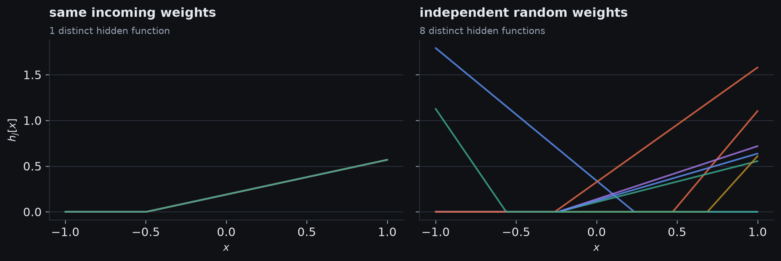
The only claim here is symmetry: hidden units that start with identical incoming weights remain one function, whereas independently initialised units can take different roles.

Reading the tied network

• eight nominal hidden units collapse to one learned function when their initial weights are tied
• training does not spontaneously give them different jobs because their gradients are the same
• different initial weights give the units different starting functions

Requirement 1: hidden units must not all start identically.

• the tied example uses the same non-zero constant rather than literal zeros, so the failure cannot be blamed on ReLU at exactly zero
• both examples use zero biases: zero biases are fine once the incoming weights differ

Candidate 2: just use random numbers

Random weights solve the symmetry problem.

A programmer’s first attempt might be something like:

weight = Math.random()

which samples values in \([0,1)\).

That gives different weights, but it also gives:

• only positive values
• a non-zero centre
• an arbitrary scale

We can centre the distribution:

weight = 2 * Math.random() - 1

Now the signs are balanced, but why should \([-1,1)\) be the right size?

Random fixes symmetry, not scale

Independent random weights are the standard way to give hidden units different starts, but randomness itself is not the mathematical requirement: the requirement is that symmetric units do not start identically.

Once we choose random, zero-centred weights, we still have to choose their scale:

• very small random weights
• medium random weights
• very large random weights

Those all break symmetry.

They do not produce the same signal behaviour through a deep network.

The two jobs of initialisation

1. break symmetry: hidden units must not all start identically; independent random weights are the standard solution
2. control signal scale: forward activations and backward gradients must remain usable through depth

Fan-in and fan-out

For one affine layer, two counts matter:

The two counts, side by side

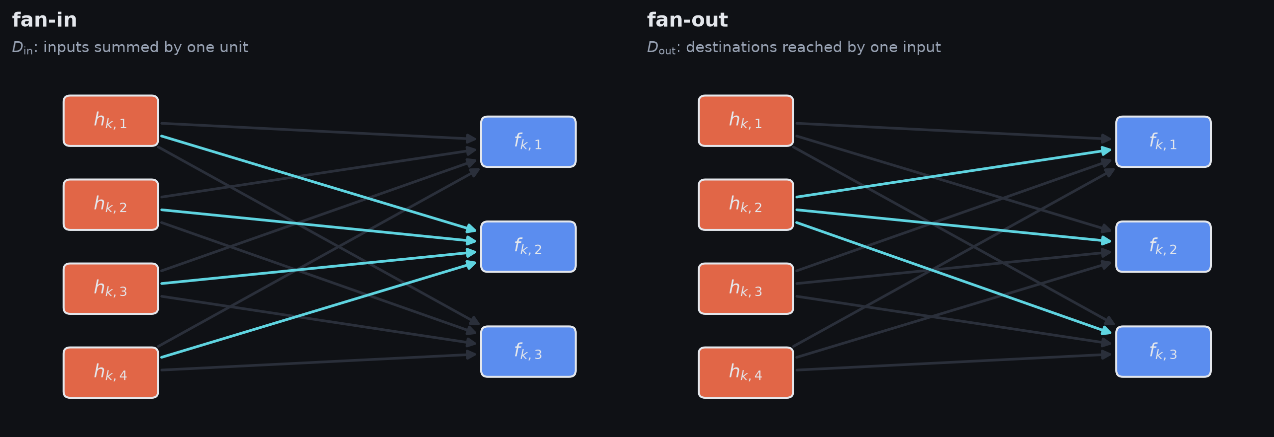
Fan-in counts the connections entering one destination unit. Fan-out counts the destinations reached by one source activation. The two counts are shown separately so the shared connection is not visually ambiguous.

Which count is which

For

\[ \mat{\Omega}_k\in\mathbb{R}^{D_{\mathrm{out}}\times D_{\mathrm{in}}}, \]

• fan-in \(D_{\mathrm{in}}\) is the number of columns
• fan-out \(D_{\mathrm{out}}\) is the number of rows

Forward signal scale depends on fan-in because one destination sums that many incoming contributions.

Backward signal scale depends on fan-out because one earlier unit collects sensitivity from that many downstream units.

Signal spread: \(\sigma\) and \(\sigma^2\)

• \(\sigma\) is the standard deviation: an ordinary measure of the signal’s spread
• \(\sigma^2\) is the variance: the squared spread
• we work mainly with variance because independent contributions add cleanly on the variance scale

The initialisation question is whether each layer systematically shrinks or grows that spread.

One layer should hand on a usable signal

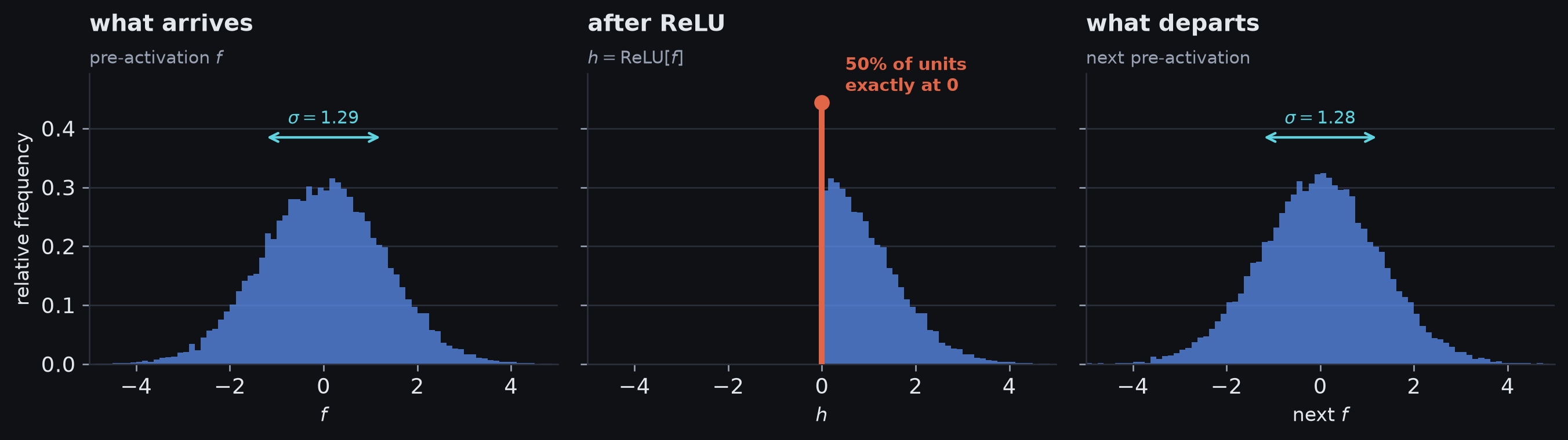
A useful initial scale lets a layer transform the signal without systematically narrowing or widening it. ReLU changes the shape, but the next affine map restores a comparable overall spread.

The engineering target

The first engineering target is simple:

a layer should not systematically hand the next layer a much smaller or much larger signal than it received

The correct random scale must therefore depend on what the layer does to the signal.

Shrinking and growing signals

Assume zero biases and independent zero-mean weights with variance \(\sigma_\Omega^2\). The effect of that variance depends on the layer width: the same \(\sigma_\Omega^2\) can be too small for one fan-in and too large for another.

Gain compounding through six layers

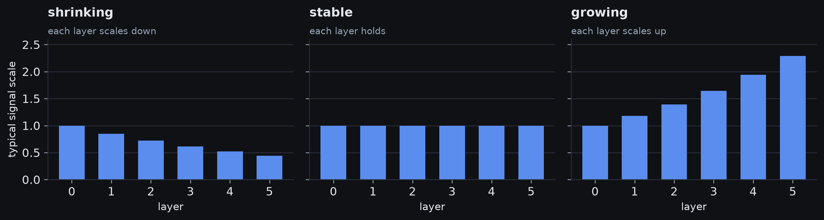
Each layer roughly multiplies signal scale by a gain factor. Repeated gains below one shrink signals, gains near one preserve them, and gains above one grow them.

• schematic, not measured: the gains are chosen to show the three regimes, and the twenty-layer figure later in this section is the measured version of the same claim

Arbitrary random scales behave differently

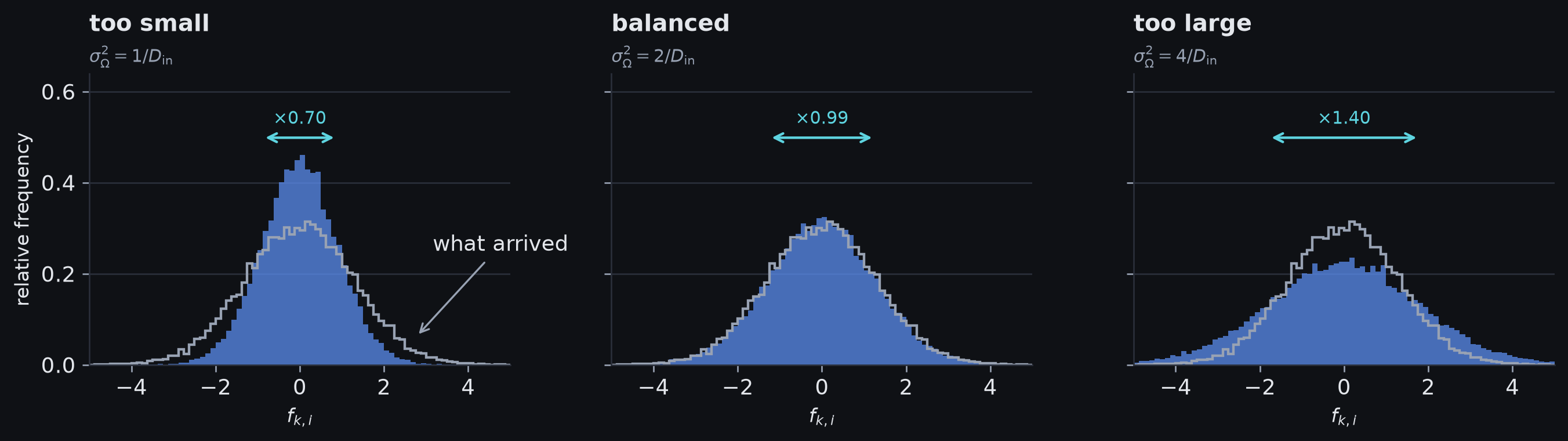
The same source activations and the same underlying random draws, scaled three ways. Randomness breaks symmetry in every panel; only the scale determines whether the signal shrinks, survives, or grows.

What each scale does to the signal

All three choices are random and zero-centred.

• too small → each layer returns less scale than it received
• balanced → scale stays comparable
• too large → each layer amplifies the signal

Randomness fixed the symmetry problem. The remaining question is how large the random weights should be.

Why fan-in changes the answer

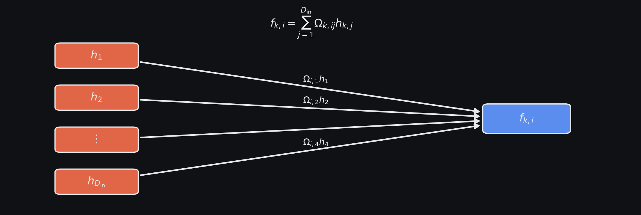
One destination pre-activation is the sum of one weighted contribution from every incoming connection. Increasing fan-in increases the number of random contributions being combined.

Fan-in 10 against fan-in 1000

A layer with fan-in \(1000\) sums one hundred times as many contributions as a layer with fan-in \(10\).

The same weight scale cannot be expected to behave identically in both.

Many random terms spread as a square root

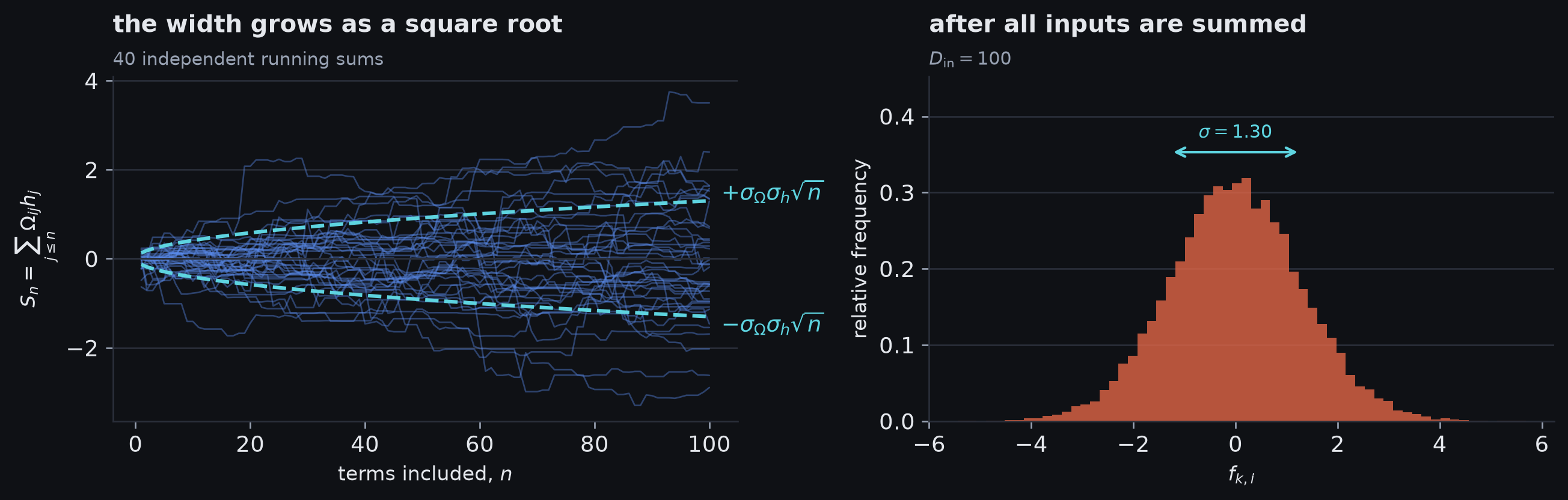
Independent zero-centred contributions partly cancel. As more terms are added, the typical width of the sum grows like the square root of the number of terms, not in direct proportion to the count.

Reading the square-root growth

• \(n\) independent centred contributions make the standard deviation grow like \(\sqrt{n}\)
• equivalently, the variance grows like \(n\)

So if fan-in multiplies the variance by roughly \(D_{\mathrm{in}}\), the weight variance needs a compensating factor proportional to

\[ \frac{1}{D_{\mathrm{in}}}. \]

Equivalently, the weight standard deviation scales like \(1/\sqrt{D_{\mathrm{in}}}\).

• one line only, and only if the room is with you: this same square-root argument is why attention divides by \(\sqrt{d_k}\) in week 5 – name it and move on, DO NOT open the topic here

The activation changes the scale too

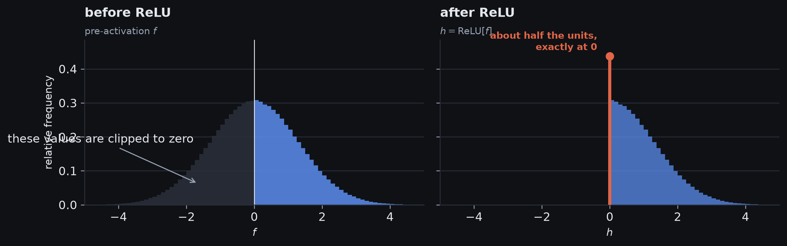
ReLU clips every negative pre-activation to zero and leaves positive values untouched. For a symmetric input, about half of the units become exactly zero.

Two effects to compensate

The initialiser therefore has to compensate for two effects:

1. fan-in combines many random contributions
2. ReLU deletes the negative half of a symmetric signal

Second moment = average squared magnitude

To track typical squared signal size, use

\[ \expect{f^2} = \text{average of the squared magnitudes of }f. \]

The formal name for this quantity is the second moment.

Squared magnitudes, before and after ReLU

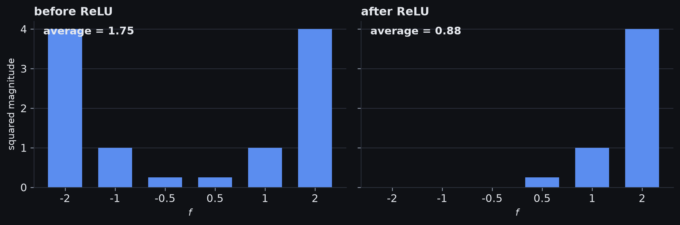
For symmetric pairs, the negative and positive values contribute equally to average squared magnitude. ReLU deletes the negative member of every pair, leaving half of that squared contribution.

The ReLU half-factor

For a distribution symmetric about zero,

\[ \boxed{ \expect{h^2}=\frac12\expect{f^2} } \qquad h=\relu(f). \]

• teach “average squared magnitude” first and “second moment” second
• do not say ReLU halves the variance: after ReLU the mean is no longer zero

So what random scale should a ReLU layer use?

Fan-in gives a factor of roughly \(D_{\mathrm{in}}\) in variance.

ReLU leaves roughly one-half of the squared magnitude.

To balance those effects, choose

\[ \boxed{ \sigma_\Omega^2 = \frac{2}{D_{\mathrm{in}}} } \qquad\Longleftrightarrow\qquad \sigma_\Omega = \sqrt{\frac{2}{D_{\mathrm{in}}}}. \]

This is He initialisation, also called Kaiming initialisation, for ReLU-style rectifiers.

• Hé is the Mandarin surname, with a rising second tone — not English he
• PyTorch uses Kaiming He’s given name: kaiming_normal_ and kaiming_uniform_

• this is the practical answer before the compact proof
• PyTorch’s usual mode="fan_in" targets forward signal preservation; mode="fan_out" targets backward signal preservation

Initialisation families

The appropriate scaling rule depends on the activation and the assumptions used to model signal propagation.

family	scaling emphasis	connection to this lecture
LeCun	fan-in based	related variance-scaling family under different activation assumptions
Glorot / Xavier	balances fan-in and fan-out	another widely used signal-preserving rule
He / Kaiming	accounts for rectifier behaviour	derived here for ReLU

Match the initialiser to the activation and architecture.

• orientation only: do not derive LeCun or Glorot here
• the purpose of naming them is to prevent He/Kaiming being learned as a universal neural-network constant

The signal model at initialisation

For one ReLU layer,

\[ f_{k,i} = \sum_{j=1}^{D_{\mathrm{in}}} \Omega_{k,ij}h_{k,j}. \]

Use a deliberately simple model of the signal at initialisation:

• biases start at zero
• weights are independent, zero-centred, and have variance \(\sigma_\Omega^2\)
• the current layer’s weights are independent of the activations arriving from the previous layer
• incoming units have approximately the same second moment
• pre-activations are approximately symmetric about zero

• the cross terms vanish in expectation under the zero-centred independence assumptions; derive the two-term expansion on the board only if useful

The forward derivation in three factors

Then the variance scale is controlled by three factors:

\[ \underbrace{D_{\mathrm{in}}}_{\text{fan-in terms}} \times \underbrace{\sigma_\Omega^2}_{\text{weight variance}} \times \underbrace{\frac12}_{\text{ReLU leaves half the squared magnitude}}. \]

• narrate the equation left to right: how many contributions, how large each weight is, how much squared magnitude ReLU leaves

The forward variance rule

So

\[ \boxed{ \var{f_{k,i}} \approx \frac12D_{\mathrm{in}}\sigma_\Omega^2 \var{f_{k-1,j}} }. \]

Setting the multiplicative gain to one gives

\[ \boxed{\sigma_\Omega^2=\frac{2}{D_{\mathrm{in}}}.} \]

Chapter 7, equation 7.32 (Prince 2023)

Fan-out controls the backward sum

Backpropagation uses

\[ \sensitivity_{k-1} = \indicator{\vect{f}_{k-1}>0} \odot \left(\layerweights_k\transpose\sensitivity_k\right). \]

For one earlier unit,

\[ \delta_{k-1,j} = \indicator{f_{k-1,j}>0} \sum_{i=1}^{D_{\mathrm{out}}} \Omega_{k,ij}\delta_{k,i}. \]

The architectural count has changed:

• forward: one destination sums fan-in contributions
• backward: one earlier unit collects fan-out contributions

Backward scale

Use a mean-field approximation for the backward signal: track the typical squared size across many units while ignoring some detailed correlations between them.

• downstream sensitivities are treated as roughly zero-centred with a common scale
• the ReLU mask is active for about half the units
• the mask is treated as sufficiently independent of the weighted downstream sum

Then

\[ \boxed{ \var{\delta_{k-1,j}} \approx \frac12D_{\mathrm{out}}\sigma_\Omega^2 \var{\delta_{k,i}} }. \]

The two meanings of the half

The factor \(1/2\) now has a different meaning:

• forward: ReLU leaves half the squared magnitude
• backward: the ReLU derivative mask is active for about half the units

Keeping backward variance stable gives

\[ \boxed{ \sigma_\Omega^2=\frac{2}{D_{\mathrm{out}}}. } \]

Chapter 7, equation 7.33 (Prince 2023)

• describe this explicitly as a mean-field-style initialisation approximation
• the ReLU mask is treated as sufficiently independent of the weighted downstream sum for this scale calculation; it is not an exact identity after training

Forward and backward targets

For a ReLU layer:

direction	architectural count	stable-variance target
forward	fan-in \(D_{\mathrm{in}}\)	\(2/D_{\mathrm{in}}\)
backward	fan-out \(D_{\mathrm{out}}\)	\(2/D_{\mathrm{out}}\)

For an equal-width layer, fan-in = fan-out, so the same Kaiming/He scale serves both directions.

For a rectangular layer, the two targets differ.

Twenty equal-width layers

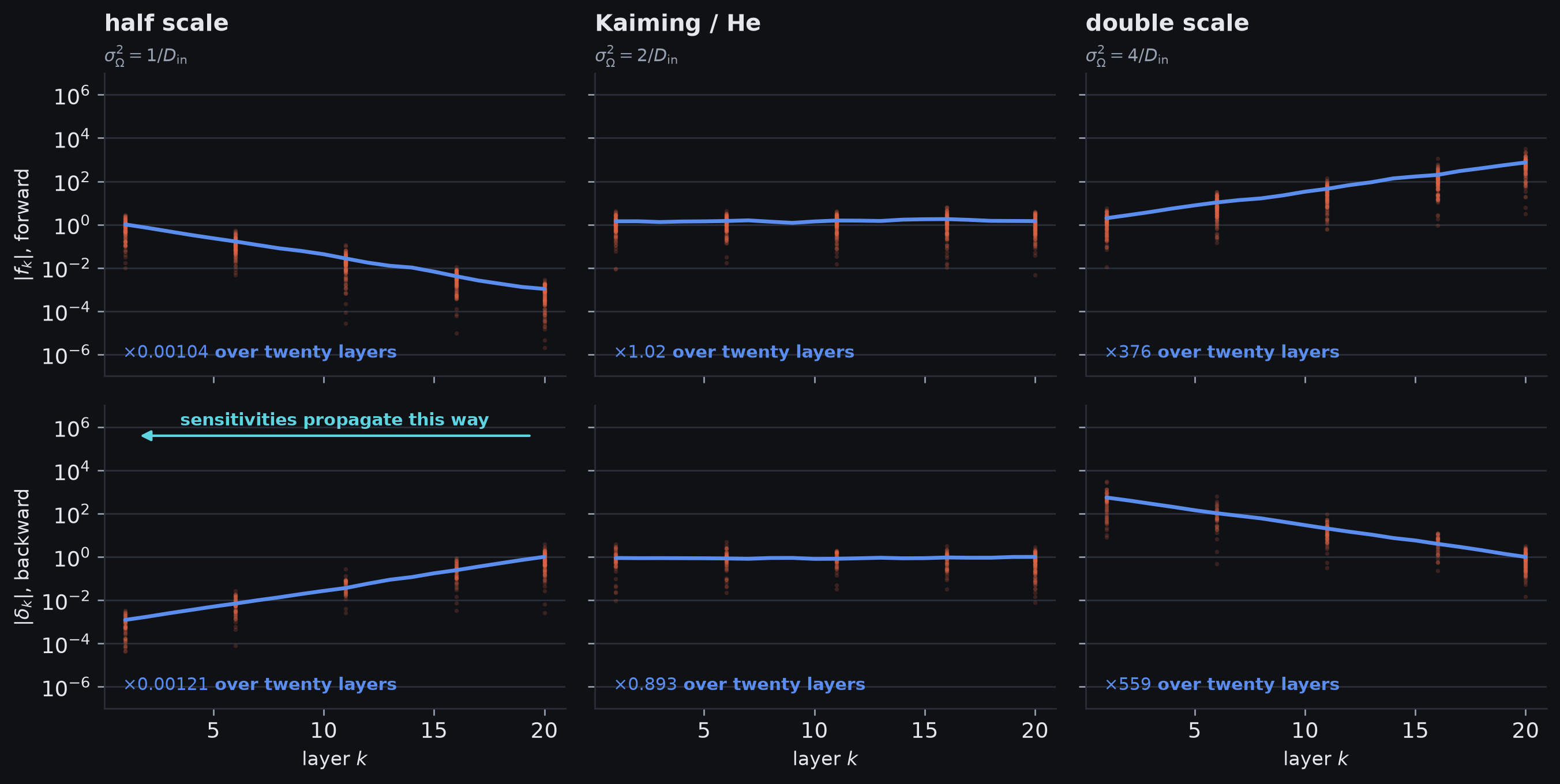
Twenty equal-width ReLU layers run forward and backward at three weight scales. Because fan-in equals fan-out here, the middle Kaiming/He scale targets both directions at once.

Reading the three columns

• too small: scale collapses repeatedly with depth
• Kaiming / He: forward and backward scales stay in the same order of magnitude
• too large: scale grows repeatedly with depth

Per-layer scaling errors compound with depth.

Rectangular layers

When

\[ D_{\mathrm{in}}\ne D_{\mathrm{out}}, \]

the exact forward and backward targets differ:

\[ \frac{2}{D_{\mathrm{in}}} \qquad\text{versus}\qquad \frac{2}{D_{\mathrm{out}}}. \]

Chapter 7 gives a symmetric compromise using the mean of the two widths:

\[ \boxed{ \sigma_\Omega^2 = \frac{4}{D_{\mathrm{in}}+D_{\mathrm{out}}}. } \]

Chapter 7, equation 7.34 (Prince 2023)

It lies between the two targets; it does not make both gains exactly one.

PyTorch’s Kaiming functions instead let the caller choose whether to preserve the fan-in / forward scale or the fan-out / backward scale.

Initialisation summary

Start with the rejected alternatives:

1. all equal → hidden units stay tied
2. arbitrary random → symmetry is broken, but signal scale is uncontrolled
3. scaled random → different units, with a scale chosen for the layer and activation

For the ReLU networks used here:

• fan-in explains the forward scaling pressure
• fan-out explains the backward scaling pressure
• under the symmetric initialisation model, ReLU supplies the half-factor that leads to the \(2\)
• Kaiming/He is the resulting ReLU-specific family
• LeCun and Glorot/Xavier are related schemes built around different propagation assumptions

A complete training step

Model, initialisation, loss, optimiser

A minimal training setup combines the derivation with the framework operations:

model = nn.Sequential(
    nn.Linear(D_i, D_h),
    nn.ReLU(),
    nn.Linear(D_h, D_h),
    nn.ReLU(),
    nn.Linear(D_h, D_o),
)

# Kaiming/He is used only where ReLU follows the linear layer.
for layer in (model[0], model[2]):
    nn.init.kaiming_normal_(layer.weight, mode="fan_in", nonlinearity="relu")
    nn.init.zeros_(layer.bias)

# No ReLU follows the output layer, so leave its weight at the framework default.
nn.init.zeros_(model[4].bias)

criterion = nn.MSELoss()
optimizer = torch.optim.SGD(model.parameters(), lr=learning_rate)

What the loss and optimiser choices commit to

• nn.MSELoss() uses mean reduction by default, averaging over all loss elements
• for scalar outputs, that divides the batch-sum gradient by the batch size; for vector outputs it divides by the total number of loss elements
• nn.MSELoss(reduction="sum") matches the batch-sum equations directly
• plain SGD matches the update rule derived in this lecture; momentum would introduce an additional optimiser state and a different update equation

Where the initialisation rule applies

PyTorch calls the Kaiming/He rule kaiming_*; here mode="fan_in" matches the forward-pass derivation above for the two ReLU hidden layers. The linear output layer deliberately does not receive that ReLU-specific rule.

Initialisation happens once; backpropagation happens on every training iteration.

The repeated training loop

for x_batch, y_batch in data_loader:
    optimizer.zero_grad()
    prediction = model(x_batch)
    loss = criterion(prediction, y_batch)
    loss.backward()
    optimizer.step()

One iteration therefore contains:

1. forward pass
2. loss evaluation
3. backward pass
4. parameter update

Activation memory

The forward pass must retain values required later by the backward pass. For a large network and batch, stored activations can dominate memory use. Two ways to trade compute or batch granularity for memory are:

• gradient checkpointing: store only selected activations and recompute missing ones during backward
• micro-batching: split a batch into smaller pieces; under the sum convention, add the sub-batch gradients, while mean-reduced gradients must be reweighted by the number of loss elements before combining

Both preserve the same underlying derivative computation while changing when intermediate values are stored or recomputed.

Parameters and saved activations in a toy network

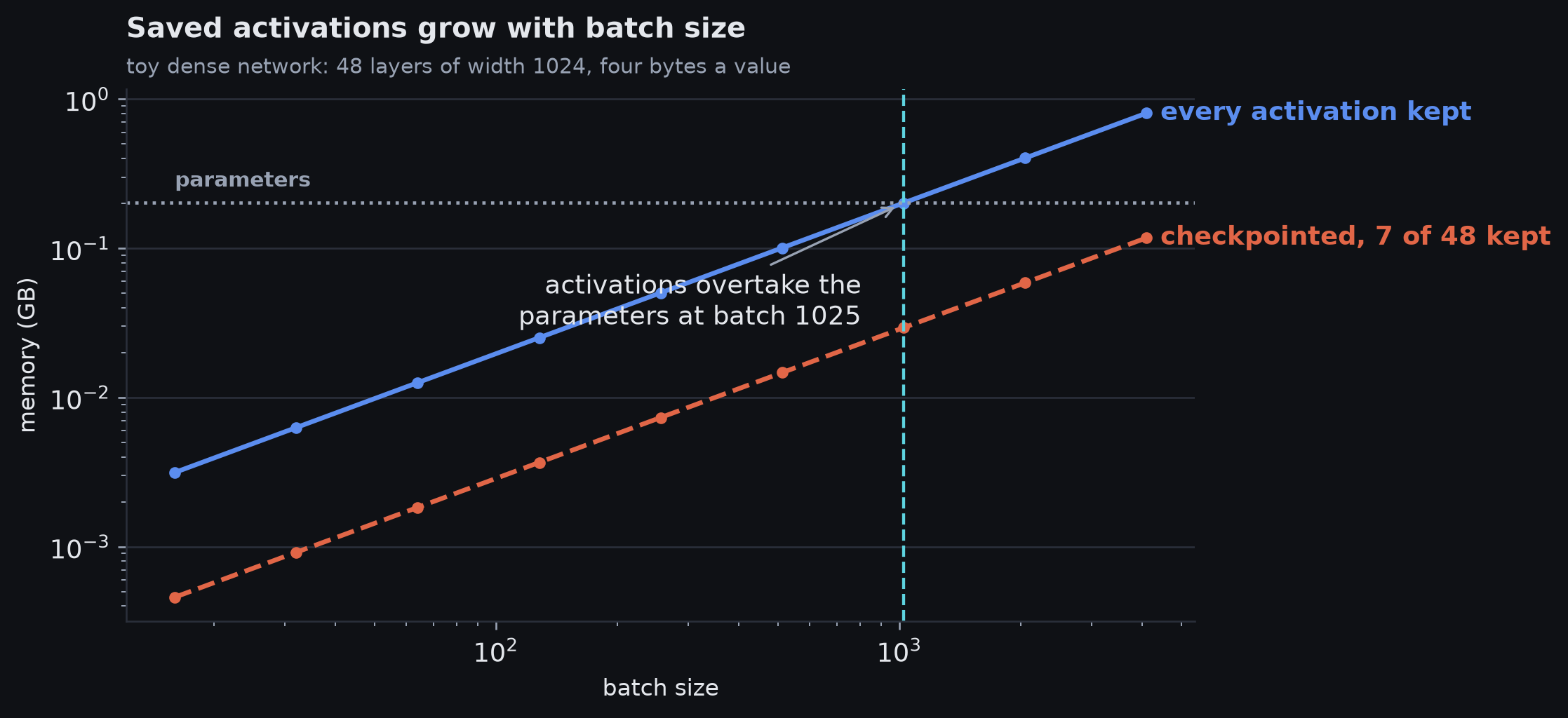
A deliberately narrow comparison of parameter storage and saved forward activations in a toy dense network. Parameter gradients, optimiser state, allocator overhead, and other framework buffers are omitted.

• counted from shapes, not quoted: a layer is one weight matrix and one bias, an activation is one value per unit per example
• the crossover lands at a batch of about the width, which is worth deriving aloud in one line
• checkpointing trades the recomputation of a forward segment for the memory of the activations inside it

Reading the memory curve

• Parameters: fixed at 0.20 GB, whatever the batch
• Activations: proportional to the batch throughout, reaching 0.81 GB at batch 4,096
• The crossover: batch 1025, which for this network is its width
• Checkpointing: the same batch stores 0.12 GB of these activations, keeping 7 layers of 48
• Not shown: parameter gradients, optimiser state, allocator/framework overhead, temporary workspaces

Checkpointing trades additional forward computation for lower activation memory.

Summary

Training computation

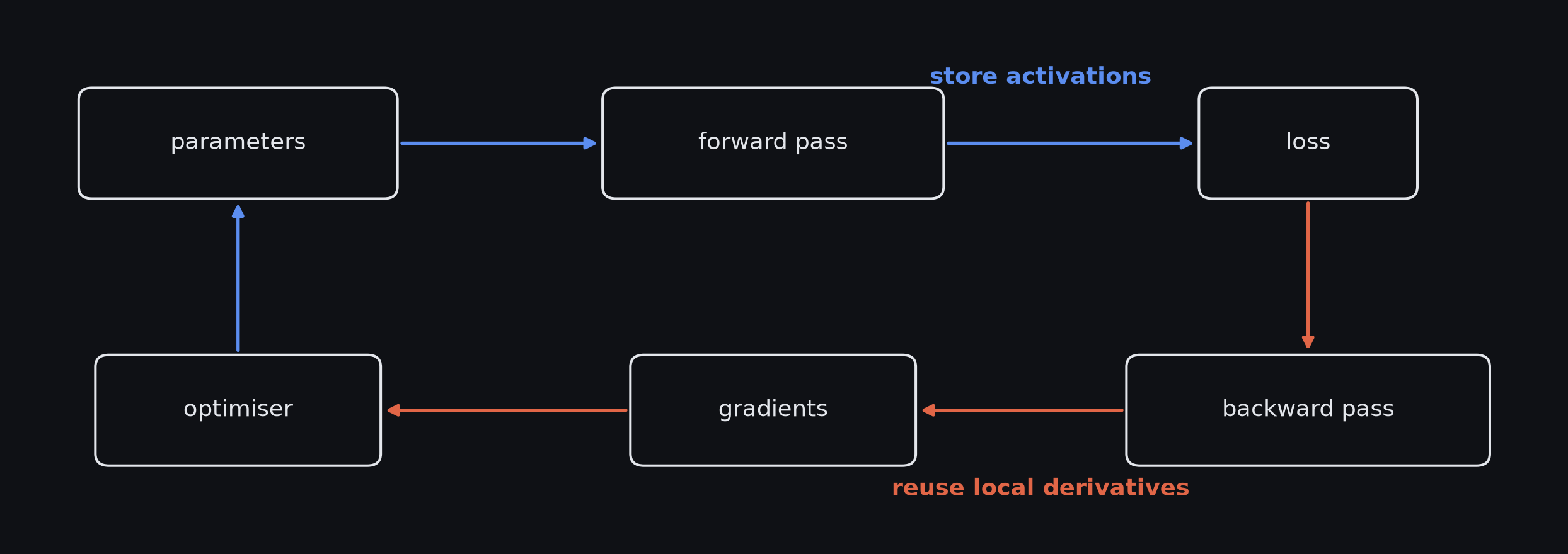
Training alternates a forward numerical computation with a backward sensitivity computation, then the optimiser converts the resulting parameter gradients into an update.

Core equations

For one example:

\[ \sensitivity_k = \nabla_{\vect{f}_k}\exloss_i \]

\[ \nabla_{\layerbias_k}\exloss_i = \sensitivity_k \]

\[ \nabla_{\layerweights_k}\exloss_i = \sensitivity_k\hidden_k\transpose \]

\[ \sensitivity_{k-1} = \indicator{\vect{f}_{k-1}>0} \odot \left( \layerweights_k\transpose\sensitivity_k \right) \]

Initialisation equations

Under the initialisation approximations stated in the derivation, for a ReLU layer,

\[ \var{f_{k,i}} \approx \frac12D_{\mathrm{in}}\sigma_\Omega^2\, \var{f_{k-1,j}}. \]

Forward scale is preserved by

\[ \boxed{\sigma_\Omega^2=\frac{2}{D_{\mathrm{in}}}.} \]

Backward scale is preserved approximately by

\[ \boxed{\sigma_\Omega^2=\frac{2}{D_{\mathrm{out}}}.} \]

For unequal fan-in and fan-out, Chapter 7 gives the compromise

\[ \boxed{\sigma_\Omega^2=\frac{4}{D_{\mathrm{in}}+D_{\mathrm{out}}}.} \]

Training pipeline

• the optimiser needs parameter gradients
• the chain rule expresses those gradients as products of local sensitivities
• deep networks contain large amounts of repeated downstream derivative work
• backpropagation reuses that work by accumulating sensitivities in reverse
• automatic differentiation packages the same mechanism into local derivative rules
• initialisation controls the scale of the quantities that flow through both passes
• Kaiming/He initialisation chooses the ReLU weight variance so that layerwise variance gain is approximately one

Source and reading

Primary reading:

• Simon J. D. Prince, Understanding Deep Learning, Chapter 7, Gradients and Initialisation (Prince 2023)

Associated notebooks:

• 7_1_Backpropagation_in_Toy_Model
• 7_2_Backpropagation
• 7_3_Initialization

Useful locators for revision:

• backpropagation recurrence: equation 7.25
• Kaiming/He forward-variance rule: equation 7.32
• backward fan-out rule: equation 7.33
• forward/backward compromise: equation 7.34
• symmetry breaking: problem 7.15

Prince, Simon J. D. 2023. Understanding Deep Learning. MIT Press. https://udlbook.github.io/udlbook/.