Lecture 4: Fitting Models

Block 4.2 Advanced AI

Eoin O’Brien

Fitting as optimisation

Recap

• A neural network is a family of functions indexed by its parameters
• A loss turns the quality of one particular parameter setting into one scalar number
• Training asks a new question:

How should we change the parameters so that this number gets smaller?

derivative → partial derivative → gradient → curvature → optimiser.

Learning goals

By the end of this lecture, you should be able to:

• explain training as optimisation in parameter space
• interpret a partial derivative as a local sensitivity
• read \(\nabla_{\params}\loss\) and explain why the gradient gives a downhill update direction
• use the chain rule to derive a simple loss gradient
• compute the gradient of least squares in both scalar and vector form
• interpret the Jacobian as a local linear map
• interpret Hessian eigenvectors and eigenvalues as principal curvature directions and curvatures
• compare gradient descent, SGD, momentum, and Adam conceptually

The fitting problem

Suppose a model predicts

\[ \hat{\vect{y}} = \vmodel{\vect{x}}, \]

where \(\params\) contains all trainable parameters.

A loss function assigns one scalar to the model’s performance on the training data:

\[ \loss[\params]. \]

Training means searching for

\[ \hat{\params} = \argmin_{\params} \loss[\params]. \]

In optimisation texts, \(\loss\) is often called the objective function. In machine learning, loss and cost are also common. Here, the objective is to minimise the loss.

What does \(\argmin\) mean?

The expression

\[ \hat{\params} = \argmin_{\params} \loss[\params] \]

is easier to read from the inside out.

• \(\loss[\params]\): how bad is this parameter setting?
• \(\min\): find the smallest achievable loss
• \(\argmin\): return the argument — the parameter values — that achieve it
• \(\hat{\params}\): our fitted estimate of those parameters

The optimiser changes parameters. Those parameters determine the predictions, and the predictions determine the loss.

Parameter vectors

For a model with two parameters,

\[ \params = \begin{bmatrix} \phi_0\\\\ \phi_1 \end{bmatrix}, \]

one parameter setting is one point in a two-dimensional parameter space.

The loss assigns a height to every point:

\[ (\phi_0,\phi_1) \longmapsto \loss[\phi_0,\phi_1]. \]

Training can now be viewed geometrically: move through parameter space toward lower loss.

Parameter space and the loss surface

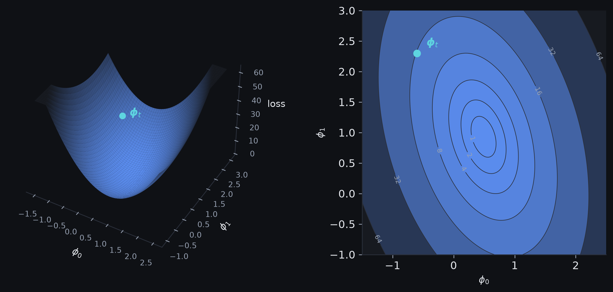
Each parameter setting is a point in parameter space; the loss assigns a height to that point.

• Emphasise: one parameter setting is one point; the loss supplies its height
• Reuse this same geometry when introducing gradients, valleys, minima, and line search

Calculus for optimisation

Average slope

Suppose we move from \(z_0\) to \(z_0+\Delta z\).

The function changes by

\[ \Delta g = g(z_0+\Delta z)-g(z_0). \]

Over that interval, the average slope is

\[ \frac{\Delta g}{\Delta z} = \frac{g(z_0+\Delta z)-g(z_0)}{\Delta z}. \]

As the interval shrinks, the secant slope approaches the local slope at \(z_0\).

Local slope

For a scalar function \(g(z)\),

\[ \frac{dg}{dz}\bigg|_{z_0} = \lim_{\Delta z\to 0} \frac{g(z_0+\Delta z)-g(z_0)}{\Delta z}. \]

The limit says: measure the slope over smaller and smaller intervals around \(z_0\).

For this lecture, the important result is the value of that local slope — not the formal machinery of limits.

Secant to tangent

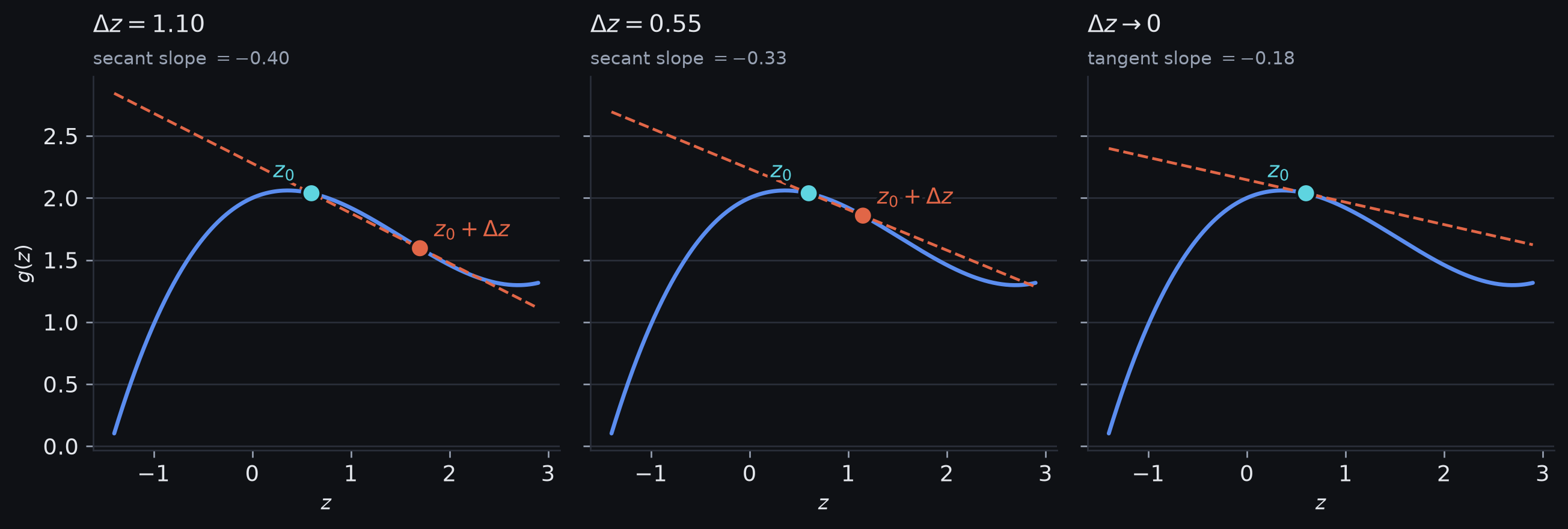
As the second point moves toward \(z_0\), the secant slope approaches the tangent slope: the derivative at \(z_0\).

• Use the familiar school-level language of slope before returning to derivative notation
• Point out the secant approaching the tangent as \(\Delta z\to0\)

First-order prediction

For a sufficiently small step \(\Delta z\),

\[ \frac{\Delta g}{\Delta z} \approx \frac{dg}{dz}\bigg|_{z_0}. \]

Multiply by \(\Delta z\):

\[ \underbrace{\Delta g}_{\text{predicted change}} \approx \underbrace{\frac{dg}{dz}\bigg|_{z_0}}_{\text{change per unit}} \underbrace{\Delta z}_{\text{proposed step}}. \]

Using the local slope

For example, if the local slope is \(3\) and \(\Delta z=0.1\),

\[ \Delta g\approx 3\times 0.1=0.3. \]

Since \(\Delta g=g(z_0+\Delta z)-g(z_0)\),

\[ \boxed{ g(z_0+\Delta z) \approx g(z_0) + \frac{dg}{dz}\bigg|_{z_0}\Delta z } \]

The derivative gives the local slope and, for a small step, predicts the change.

Tangent-line approximation

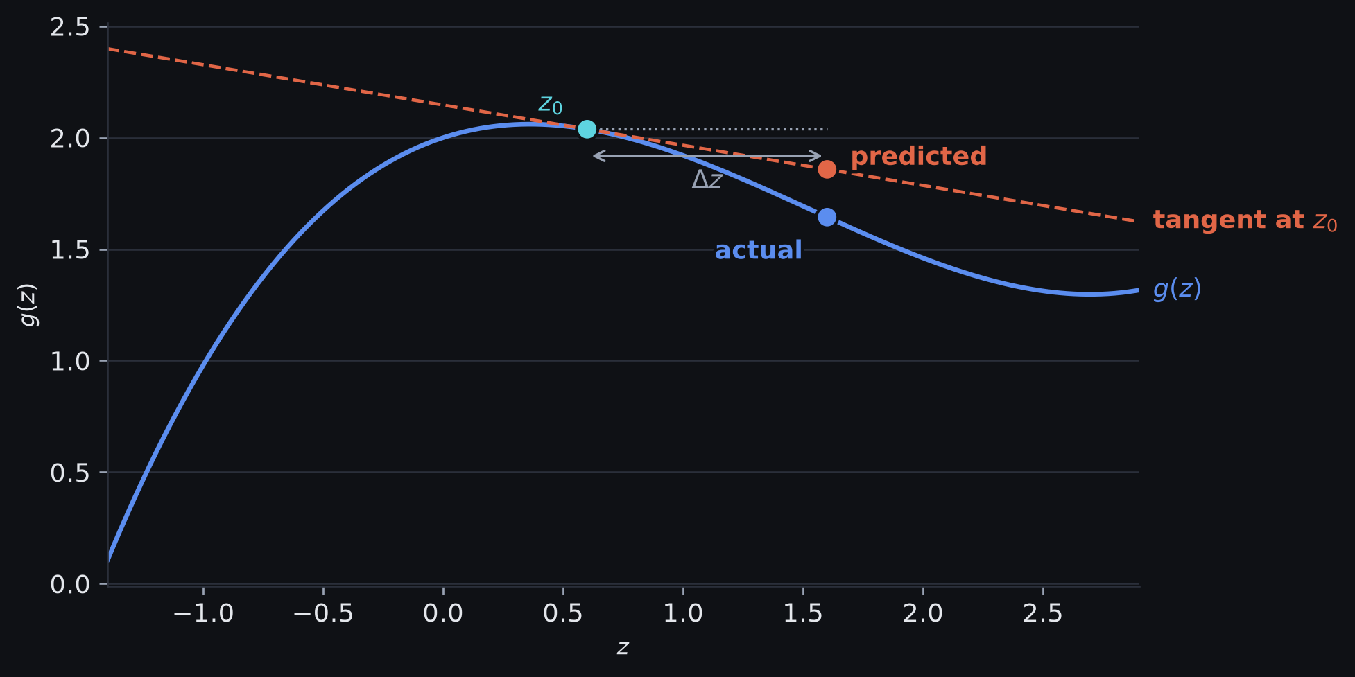
Near \(z_0\), the tangent line uses the derivative to predict the effect of a small input change \(\Delta z\).

• Emphasise: the tangent is a local linear approximation
• Reuse this approximation when moving to several parameters

Many parameters

A neural network does not have one parameter.

It may have millions or billions:

\[ \params = [\phi_0,\phi_1,\ldots,\phi_N]\transpose. \]

With many parameters, ask the derivative question one coordinate at a time:

What happens to the loss if I nudge this parameter while temporarily holding the others fixed?

This is a partial derivative.

Partial derivatives

For a loss \(\loss[\phi_0,\phi_1]\),

\[ \frac{\partial \loss}{\partial \phi_0} \]

means:

• vary \(\phi_0\) slightly
• hold \(\phi_1\) fixed
• measure the local rate of change of the loss

Likewise,

\[ \frac{\partial \loss}{\partial \phi_1} \]

asks the same question along the other coordinate direction.

Partial-derivative notation

Notation:

• \(d\) is used above for a function with one independent variable
• \(\partial\) reminds us that \(\loss\) depends on several parameters and we are varying only one

Read \(\partial\loss/\partial\phi_0\) as “partial L with respect to phi-zero.”

Partial derivatives as slices

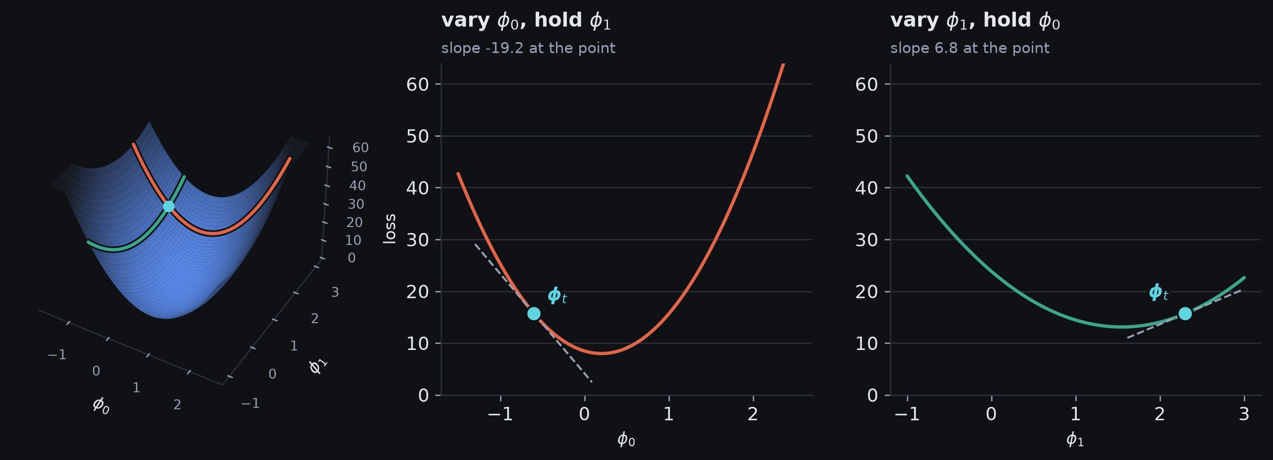
Each partial derivative measures the local slope along one parameter axis while the other parameters are held fixed.

• Point out that only one coordinate changes in each slice
• Contrast one coordinate sensitivity with the full gradient vector

The gradient

One partial derivative tells us about one coordinate.

The gradient collects all coordinate sensitivities in one vector:

\[ \boxed{ \nabla_{\params}\loss = \begin{bmatrix} \dfrac{\partial \loss}{\partial \phi_0}\\[0.6em] \dfrac{\partial \loss}{\partial \phi_1}\\ \vdots\\ \dfrac{\partial \loss}{\partial \phi_N} \end{bmatrix} } \]

\(\nabla\) is nabla.

Read \(\nabla_{\params}\loss\) as “the gradient of the loss with respect to the parameters.”

Its shape matches \(\params\): one sensitivity for every parameter.

First-order change in parameter space

Suppose we change all parameters by a small vector \(\Delta\params\).

The scalar prediction rule becomes

\[ \boxed{ \loss[\params+\Delta\params] \approx \loss[\params] + \inner{\nabla_{\params}\loss}{\Delta\params} } \]

The dot product adds the predicted contribution from every coordinate:

\[ \inner{\nabla_{\params}\loss}{\Delta\params} = \frac{\partial\loss}{\partial\phi_0}\Delta\phi_0 + \frac{\partial\loss}{\partial\phi_1}\Delta\phi_1 + \cdots + \frac{\partial\loss}{\partial\phi_N}\Delta\phi_N. \]

Steepest ascent and descent

For parameter moves with the same Euclidean length,

\[ \inner{\nabla_{\params}\loss}{\Delta\params} \]

is largest when \(\Delta\params\) points in the same direction as the gradient.

Using the angle form of the dot product from week 1:

\[ \inner{\nabla_{\params}\loss}{\Delta\params} = \norm{\nabla_{\params}\loss}\,\norm{\Delta\params}\cos\theta. \]

• at the current point, \(\norm{\nabla_{\params}\loss}\) is fixed
• comparing equal-length moves fixes \(\norm{\Delta\params}\)
• only \(\cos\theta\) varies: it is largest at \(\theta=0\) and smallest at \(\theta=\pi\)

So, under the ordinary Euclidean notion of step size, and wherever the gradient isn’t \(\vect{0}\):

• \(\nabla_{\params}\loss\) is the locally steepest uphill direction
• \(-\nabla_{\params}\loss\) is the locally steepest downhill direction

Equal-length moves

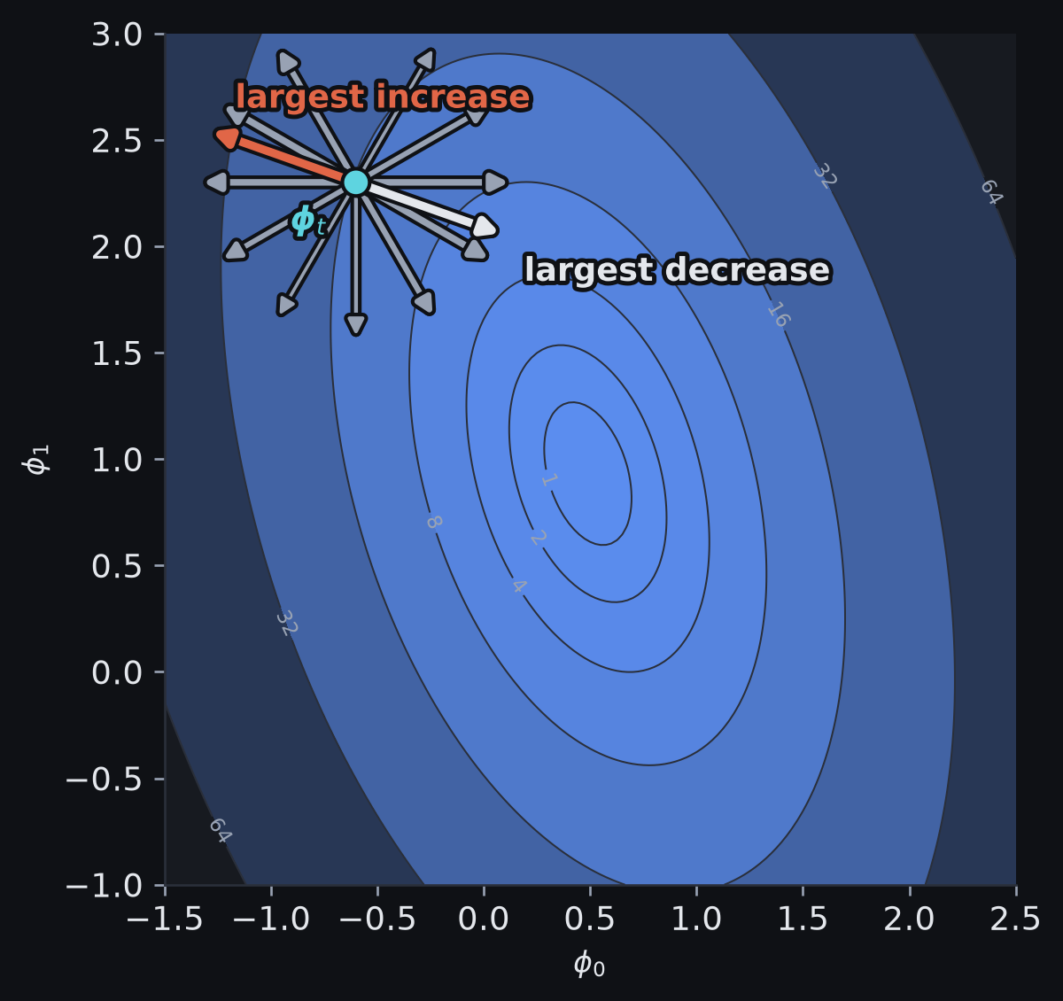
Among equal-length parameter moves, the move aligned with the gradient gives the largest predicted increase in loss; the opposite move gives the largest predicted decrease.

• Every arrow has the same Euclidean length
• Relate each predicted change to the gradient dot product
• Alignment maximises the dot product; opposite alignment minimises it

The gradient on a contour map

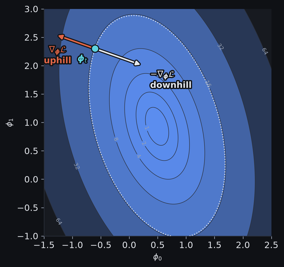
On a contour map, \(\nabla_{\params}\loss\) points in the direction of steepest local increase; \(-\nabla_{\params}\loss\) gives the steepest local decrease.

• Walk from the dot-product formula to the contour geometry
• The dotted curve is the actual equal-loss contour through the current point
• Point out that the gradient is normal to that contour at the current point

Reading the contour map

• The dotted curve is the contour through \(\params_t\): every point on it has the same loss
• The gradient is perpendicular to the contour locally, giving the steepest first-order increase
• The minus sign reverses that direction to give the steepest first-order decrease

First-order optimisation

Gradient descent

Gradient descent uses this direction directly:

\[ \underbrace{\params_{t+1}}_{\text{new parameters}} = \underbrace{\params_{t}}_{\text{current parameters}} - \underbrace{\alpha}_{\text{step size}} \underbrace{\nabla_{\params}\loss[\params_t]}_{\text{uphill direction}}. \]

• the gradient gives the local uphill direction
• the minus sign reverses it
• \(\alpha>0\) sets the step size
• the calculation is repeated at the new parameter values

Learning rate

The learning rate \(\alpha\) sets the size of each update.

Too small:

• stable updates
• slow progress

Too large:

• faster movement
• risk of overshoot, oscillation, or divergence

A classical way to choose the step length is a line search: first choose a downhill direction, then search along that line for a useful value of \(\alpha\).

Step direction and step length

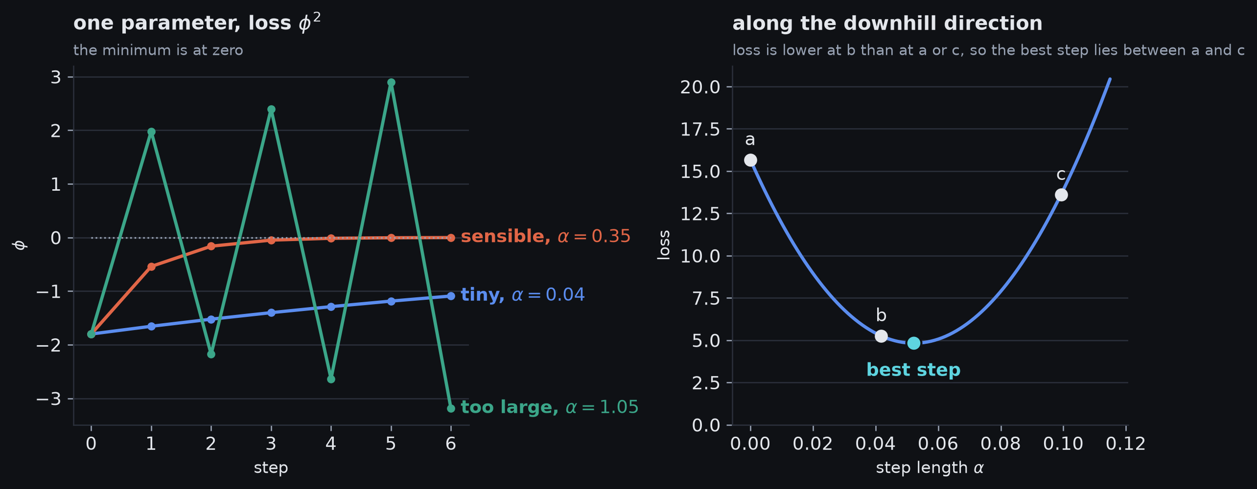
The gradient chooses a descent direction; the learning rate or line search determines how far to move along it.

• Separate direction choice from step-length choice; line search addresses the latter

Differentiating a model

Worked example: linear regression

Start with the familiar model

\[ \hat{y}_i = \model{x_i} = \phi_0+\phi_1x_i. \]

For one training example \((x_i,y_i)\), define the residual

\[ r_i = \underbrace{\phi_0+\phi_1x_i}_{\text{prediction}} - \underbrace{y_i}_{\text{target}}. \]

Week 1 wrote the residual as target minus prediction. This lecture follows Prince’s order, so the residual sign flips but the squared loss is unchanged.

With squared error,

\[ \exloss_i=r_i^2. \]

Numerical check

Take one example with

\[ x_i=2,\qquad y_i=5,\qquad \phi_0=1,\qquad \phi_1=1. \]

The model predicts \(3\), so

\[ r_i=3-5=-2,\qquad \exloss_i=(-2)^2=4. \]

Now nudge only the intercept by \(\Delta\phi_0=0.1\). The prediction rises from \(3\) to \(3.1\), so the residual becomes less negative and the squared error should fall.

The derivative predicts the size of that local change.

Chain-rule graph

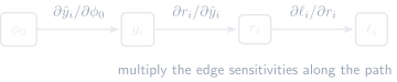
The chain rule multiplies local sensitivities along a dependency path from a parameter to the loss.

The chain rule

Learning problems are built from dependent calculations:

\[ \phi_0 \longrightarrow r_i \longrightarrow \exloss_i. \]

The chain rule multiplies the local sensitivities along that path:

\[ \boxed{ \frac{\partial\exloss_i}{\partial\phi_0} = \underbrace{\frac{\partial\exloss_i}{\partial r_i}}_{\text{loss sensitivity}} \underbrace{\frac{\partial r_i}{\partial\phi_0}}_{\text{model sensitivity}} } \]

More generally, if changing \(a\) changes \(b\), and changing \(b\) changes \(c\),

\[ \frac{dc}{da} = \frac{dc}{db}\frac{db}{da}. \]

A deep network uses the same rule repeatedly through a much larger dependency graph.

Derivative with respect to \(\phi_0\)

We want

\[ \frac{\partial \exloss_i}{\partial \phi_0}. \]

Start from

\[ \exloss_i=(\phi_0+\phi_1x_i-y_i)^2. \]

Use the chain rule:

\[ \frac{\partial \exloss_i}{\partial \phi_0} = \underbrace{2r_i}_{\text{how loss changes with residual}} \underbrace{\frac{\partial r_i}{\partial \phi_0}}_{=1} = 2r_i. \]

The intercept derivative is proportional to the signed residual.

Derivative with respect to \(\phi_1\)

For the slope parameter:

\[ \frac{\partial \exloss_i}{\partial \phi_1} = \underbrace{2r_i}_{\text{error signal}} \underbrace{\frac{\partial r_i}{\partial \phi_1}}_{=x_i} = 2x_i r_i. \]

Why does \(x_i\) appear?

Because changing the slope affects the prediction by an amount proportional to the input:

\[ \frac{\partial}{\partial\phi_1}(\phi_1x_i)=x_i. \]

Checking the derivative prediction

The example from earlier: \(x_i=2\), \(r_i=-2\), and a nudge of \(\Delta\phi_0=0.1\).

• Sensitivity: \(\partial\exloss_i/\partial\phi_0=2r_i=-4\)
• Predicted change: \(-4\times 0.1=-0.4\)
• Actual change: \((-1.9)^2-(-2)^2=-0.39\)

The derivative predicts \(-0.4\); the actual change is \(-0.39\).

Their difference is second order: halve the step and it quarters.

Per-example gradient

Stack the two partial derivatives to form the per-example gradient:

\[ \nabla_{\params}\exloss_i = \begin{bmatrix} 2r_i\\\\ 2x_i r_i \end{bmatrix} = 2r_i \begin{bmatrix} 1\\\\ x_i \end{bmatrix}. \]

The two factors have different roles:

• \(2r_i\): how wrong the model is
• \([1,x_i]\transpose\): how this example couples to the parameters

Dataset gradient

If

\[ \loss[\params] = \sum_{i=1}^{I}\exloss_i, \]

then differentiation distributes across the sum:

\[ \nabla_{\params}\loss = \sum_{i=1}^{I} \nabla_{\params}\exloss_i. \]

The full gradient is the sum of the per-example gradients.

Sum or mean?

We use a sum here because it follows directly from the per-example derivation. Many libraries report the mean loss instead:

\[ \bar{\loss}=\frac{1}{I}\sum_{i=1}^{I}\exloss_i. \]

The minimiser is unchanged; the gradient is simply scaled by \(1/I\). That constant scale can be accounted for in the learning rate.

Matrix calculus

Writing one derivative per parameter is manageable for two parameters.

With millions of parameters, coordinate-by-coordinate notation is no longer practical.

Matrix calculus expresses the same derivative relationships compactly for vectors and matrices, while keeping the structure of the computation visible.

The design matrix

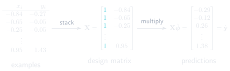
The design matrix collects all examples so that the complete prediction vector is computed as \(\mat{X}\params\).

• Emphasise that vectorisation reorganises the same computation; it does not define a new model
• Point out the bias column of ones

Linear regression in vector form

For all \(I\) examples, create the design matrix

\[ \mat{X} = \begin{bmatrix} 1 & x_1\\\\ 1 & x_2\\\\ \vdots & \vdots\\\\ 1 & x_I \end{bmatrix}, \qquad \params = \begin{bmatrix} \phi_0\\\\ \phi_1 \end{bmatrix}. \]

Stacking the examples gives all predictions in one matrix multiplication:

\[ \hat{\vect{y}} = \mat{X}\params. \]

The residual vector

The residual vector is

\[ \vect{r}=\mat{X}\params-\vect{y}. \]

• Same order as the scalar above: prediction minus target, so this is the negative of week 1’s residual vector
• the squared loss is unchanged
• the parameter gradient is unchanged when the convention is used consistently: both \(\vect{r}\) and \(\partial\vect{r}/\partial\params\) change sign

The loss in vector form

The sum of squared residuals is

\[ \loss[\params] = \sum_{i=1}^{I} r_i^2 = \vect{r}\transpose\vect{r}. \]

Substituting \(\vect{r}=\mat{X}\params-\vect{y}\):

\[ \loss[\params] = (\mat{X}\params-\vect{y})\transpose (\mat{X}\params-\vect{y}). \]

The vector expression is identical to the scalar least-squares loss.

Matrix gradient I: residual sensitivity

We already have

\[ \loss=\vect{r}\transpose\vect{r}. \]

So the loss sensitivity with respect to the residual vector is

\[ \nabla_{\vect{r}}\loss=2\vect{r}. \]

This is the vector version of \(d(r^2)/dr=2r\).

And because

\[ \vect{r}=\mat{X}\params-\vect{y}, \]

a small parameter move produces

\[ \Delta\vect{r}=\mat{X}\Delta\params. \]

Matrix gradient II: parameter sensitivity

The first-order change in loss is

\[ \Delta\loss \approx \inner{2\vect{r}}{\Delta\vect{r}} = (2\vect{r})\transpose\mat{X}\Delta\params. \]

Rearrange the scalar product:

\[ \Delta\loss \approx \left(2\mat{X}\transpose\vect{r}\right)\transpose\Delta\params. \]

Compare this with

\[ \Delta\loss\approx(\nabla_{\params}\loss)\transpose\Delta\params. \]

Both expressions must agree for every small \(\Delta\params\), so their coefficient vectors are equal:

\[ \boxed{\nabla_{\params}\loss=2\mat{X}\transpose\vect{r}=2\mat{X}\transpose(\mat{X}\params-\vect{y})}. \]

Interpreting the matrix gradient

1. \(\mat{X}\params-\vect{y}\): compute the residuals.

2. \(2(\cdot)\): convert each residual into a loss sensitivity.

3. \(\mat{X}\transpose(\cdot)\): map those sensitivities back onto the parameter coordinates.

This is the same chain rule as the one-example derivation, written for the whole dataset.

The Jacobian

Suppose a vector-valued function produces

\[ \vect{z}=\vect{f}(\params) \in\reals^{\dout}, \qquad \params\in\reals^{N+1}. \]

Its Jacobian collects every first-order sensitivity:

\[ \mat{J}_{\vect{f}} = \frac{\partial \vect{z}}{\partial \params\transpose} = \begin{bmatrix} \dfrac{\partial z_1}{\partial \phi_0} & \cdots & \dfrac{\partial z_1}{\partial \phi_N}\\\\ \vdots & \ddots & \vdots\\\\ \dfrac{\partial z_{\dout}}{\partial \phi_0} & \cdots & \dfrac{\partial z_{\dout}}{\partial \phi_N} \end{bmatrix}. \]

Our convention is: rows correspond to outputs; columns correspond to parameters. With this convention, \(\mat{J}_{\vect{f}}\) has shape \(\dout\times(N+1)\).

The Jacobian as a local linear map

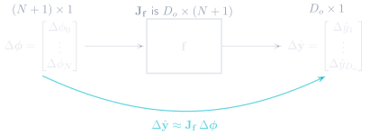
The Jacobian maps a small parameter perturbation to the corresponding first-order change in the model outputs.

• Present the Jacobian as a local linear map; the derivative table is its coordinate representation
• Emphasise that its transpose maps output sensitivities back to parameters

The Jacobian in the chain rule

A loss often has the structure

\[ \params \longrightarrow \hat{\vect{y}} \longrightarrow \loss. \]

The multivariable chain rule says

\[ \nabla_{\params}\loss = \mat{J}_{\vect{f}}\transpose \nabla_{\hat{\vect{y}}}\loss. \]

• \(\nabla_{\hat{\vect{y}}}\loss\) gives the sensitivity of the scalar loss to each output
• \(\mat{J}_{\vect{f}}\transpose\) maps those output sensitivities back to the parameters

Check the dimensions:

\[ \underbrace{\mat{J}_{\vect{f}}\transpose}_{(N+1)\times\dout} \underbrace{\nabla_{\hat{\vect{y}}}\loss}_{\dout\times 1} = \underbrace{\nabla_{\params}\loss}_{(N+1)\times 1}. \]

The same chain-rule pattern propagates loss sensitivities through a deep network.

Curvature and loss geometry

The convex case

Linear least squares has a convex loss landscape.

For a convex function, every local minimum is also global.

Geometrically, every chord joining two points on the graph lies on or above the function.

Convexity removes suboptimal local minima from the landscape.

Gradient descent still needs a suitable step-size strategy to converge.

Second derivatives

For a scalar function \(g(z)\),

\[ g'(z)=\frac{dg}{dz} \]

gives the local slope.

Differentiate the slope itself:

\[ g''(z)=\frac{d^2g}{dz^2}. \]

The second derivative measures how the slope changes as we move.

Locally:

• \(g''(z)>0\): the graph curves upward
• \(g''(z)<0\): the graph curves downward
• \(g''(z)=0\): second-order information alone may be inconclusive

The Hessian

For a scalar loss with many parameters, the gradient is itself a vector-valued function:

\[ \params \longmapsto \nabla_{\params}\loss. \]

Differentiate that vector with respect to the parameters:

\[ \boxed{ \mat{H} = \frac{\partial(\nabla_{\params}\loss)}{\partial\params\transpose} = \nabla_{\params}^{2}\loss } \]

This matrix is the Hessian.

Hessian entries

Expanded,

\[ \mat{H} = \begin{bmatrix} \dfrac{\partial^2 \loss}{\partial \phi_0^2} & \dfrac{\partial^2 \loss}{\partial \phi_0\partial\phi_1} & \cdots\\[0.8em] \dfrac{\partial^2 \loss}{\partial \phi_1\partial\phi_0} & \dfrac{\partial^2 \loss}{\partial \phi_1^2} & \cdots\\ \vdots & \vdots & \ddots \end{bmatrix}. \]

• diagonal terms: curvature along individual coordinates
• off-diagonal terms: how changing one parameter changes the slope with respect to another

To interpret the Hessian geometrically, recall how a matrix acts on directions.

Scaling

Recall that matrix multiplication can be read geometrically as a linear transformation.

Here the matrix stretches one coordinate and shrinks the other:

\[ \mat{A} = \begin{bmatrix} 1.8 & 0\\ 0 & 0.65 \end{bmatrix}. \]

Scaling the plane

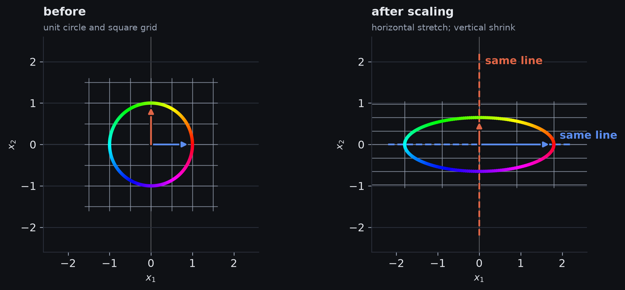
Under non-uniform scaling, the grid and unit circle stretch into a rectangle-like grid and an ellipse. The hue tracks each point from the original circle to its transformed position.

• Hue identifies where each point on the original circle went
• Ask: which directions have changed length but not line?
• Do not name eigenvectors yet; let the special directions be noticed first

Invariant lines under scaling

For this scaling matrix, horizontal and vertical vectors change length but remain on their original lines.

Rotation

Now rotate every vector by \(40^\circ\):

\[ \mat{R} = \begin{bmatrix} \cos 40^\circ & -\sin 40^\circ\\ \sin 40^\circ & \cos 40^\circ \end{bmatrix}. \]

Rotating the plane

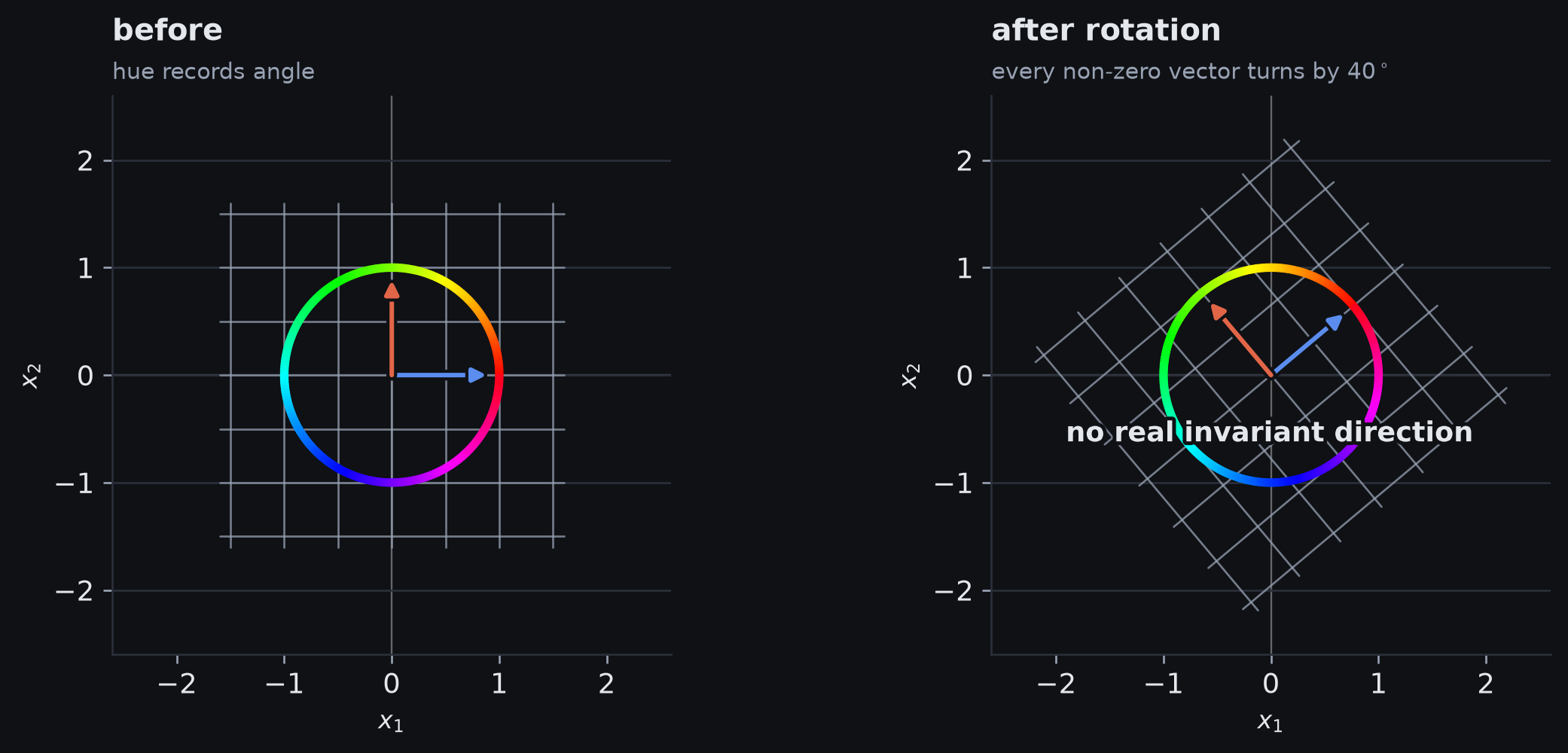
A rotation preserves the shape of the unit circle, so hue is important: every coloured point moves around the circle. No non-zero real vector remains on its original line for this angle.

• Without the hue, a rotated circle is visually indistinguishable from the original circle
• Contrast this with scaling: there, two real directions stayed on their own lines

No real invariant direction

The circle still looks like a circle, but the hue shows that every non-zero real vector has moved to a different line.

Shear

A shear mixes the coordinates:

\[ \mat{S} = \begin{bmatrix} 1 & 1.1\\ 0 & 1 \end{bmatrix}. \]

Shearing the plane

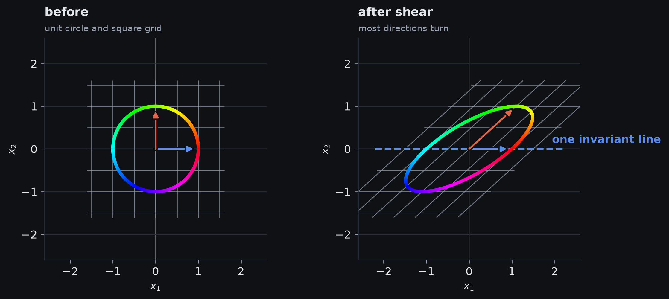
A shear tilts the grid and turns most vectors, but the horizontal axis remains on the same line.

One invariant line

Most directions turn, but vectors on the horizontal axis remain on that same line.

A real \(2\times2\) matrix therefore need not have two distinct real invariant directions.

Eigenvectors and eigenvalues

Those invariant directions are eigenvector directions.

A non-zero vector \(\vect{v}\) is an eigenvector of \(\mat{A}\) when

\[ \boxed{\mat{A}\vect{v}=\lambda\vect{v}}. \]

Geometrically:

• \(\mat{A}\vect{v}\) is a scalar multiple of \(\vect{v}\)
• for \(\lambda\ne0\), the transformed vector stays on the same line through the origin
• \(|\lambda|\) gives the scale factor; the sign gives the orientation
• any non-zero multiple of an eigenvector lies on the same eigendirection

Interpreting eigenvalues

The sign and magnitude of \(\lambda\) tell us what happened:

• \(\lambda>1\): stretch
• \(0<\lambda<1\): shrink
• \(\lambda<0\): scale and reverse orientation
• \(\lambda=0\): collapse that direction to the origin

For the scaling matrix above,

\[ \mat{A}\begin{bmatrix}1\\0\end{bmatrix} =1.8\begin{bmatrix}1\\0\end{bmatrix}, \qquad \mat{A}\begin{bmatrix}0\\1\end{bmatrix} =0.65\begin{bmatrix}0\\1\end{bmatrix}. \]

The coordinate axes are eigenvector directions; \(1.8\) and \(0.65\) are their eigenvalues.

Eigenvalues as polynomial roots

To find an eigenvector, we need a non-zero solution of

\[ (\mat{A}-\lambda\mat{I})\vect{v}=\vect{0}. \]

A non-zero solution exists only when \(\mat{A}-\lambda\mat{I}\) is singular: it must map some non-zero vector to zero.

For a square matrix, singular means determinant zero:

\[ \boxed{\det(\mat{A}-\lambda\mat{I})=0}. \]

This characteristic equation is a polynomial in \(\lambda\).

The eigenvalues are the roots of this polynomial.

As with ordinary polynomial roots, they need not all be real.

Rotation and complex eigenvalues

For a \(90^\circ\) rotation,

\[ \mat{R}_{90} = \begin{bmatrix} 0 & -1\\ 1 & 0 \end{bmatrix}, \qquad \det(\mat{R}_{90}-\lambda\mat{I}) = \lambda^2+1. \]

Its roots are \(\lambda=\pm i\), so there is no real eigendirection. That matches the geometry: every real vector turns.

Repeated eigenvalues

A repeated root need not provide the same number of independent eigenvectors.

For the shear matrix

\[ \mat{S} = \begin{bmatrix} 1 & 1.1\\ 0 & 1 \end{bmatrix}, \]

we get

\[ \det(\mat{S}-\lambda\mat{I})=(1-\lambda)^2. \]

So \(\lambda=1\) is a repeated eigenvalue, but the horizontal axis supplies only one independent real eigendirection.

Symmetric matrices

Symmetric Hessians

For the sufficiently smooth losses considered here, the mixed second partials agree, so the Hessian is symmetric.

Real symmetric matrices have:

• real eigenvalues
• a full set of mutually orthogonal eigenvector directions

For a Hessian, the eigenvectors therefore give a complete set of real principal directions.

• The rotation and shear examples showed what can go wrong for a general matrix
• Symmetry removes those complications for the Hessian: real eigenvalues and an orthogonal eigenbasis

Local change in the gradient

For a small parameter move \(\Delta\params\), the Hessian gives the first-order change in the gradient:

\[ \boxed{ \nabla_{\params}\loss[\params+\Delta\params] \approx \nabla_{\params}\loss[\params] + \mat{H}\Delta\params } \]

\(\mat{H}\Delta\params\) is the first-order predicted change in the gradient caused by the parameter move \(\Delta\params\).

Second-order loss approximation

Near the current parameters,

\[ \loss[\params+\Delta\params] \approx \loss[\params] + \underbrace{\inner{\nabla_{\params}\loss}{\Delta\params}}_{\text{first-order change}} + \frac{1}{2} \underbrace{\Delta\params\transpose\mat{H}\Delta\params}_{\text{curvature correction}}. \]

The linear term contains the local slope information; the quadratic term adds the curvature correction.

The least-squares Hessian

Recall

\[ \nabla_{\params}\loss = 2\mat{X}\transpose(\mat{X}\params-\vect{y}). \]

Differentiate once more:

\[ \mat{H} = 2\mat{X}\transpose\mat{X}. \]

The Hessian no longer depends on \(\params\): ordinary least squares has the same curvature everywhere in parameter space.

Because \(\mat{X}\transpose\mat{X}\) is positive semidefinite, the least-squares objective is convex.

• \(\vect{v}\transpose\mat{X}\transpose\mat{X}\vect{v}=\norm{\mat{X}\vect{v}}^2\ge 0\) for every \(\vect{v}\)
• full column rank makes the Hessian positive definite and the minimiser unique
• dependent columns create zero-curvature directions and can give multiple optimal minimisers

Isotropy: equal turning

The terminology comes from Greek:

• isos (ἴσος): equal
• tropos (τρόπος): a turn, way, or direction

So isotropic is literally the idea of equal turning:

turn in a different direction, and the behaviour stays the same.

Anisotropic adds a negative prefix: the behaviour is not the same in every direction.

A familiar tropos

Homer describes Odysseus as polytropos (πολύτροπος): poly, many, + tropos, turns / ways.

In Homer the epithet has a broader sense — resourceful, wily, “of many turns” — but the shared root is useful here:

polytropos → many-turning; isotropic → equal-turning.

Isotropy in parameter space

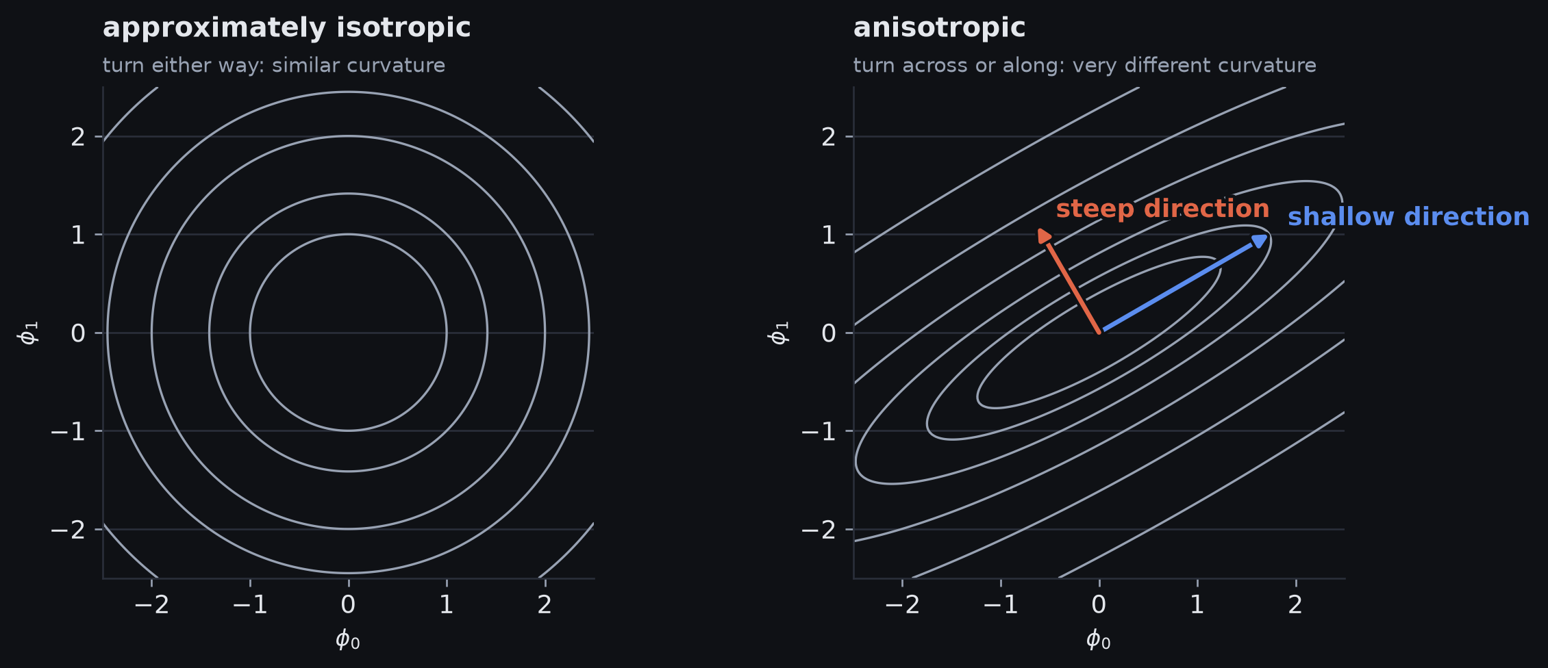
Isotropic means that turning to a different direction changes little; anisotropic means that curvature depends strongly on the direction.

• Pronounce only the useful roots: isos = equal; tropos = turn / way / direction
• Connect tropos to Odysseus as polytropos; note that the Homeric epithet has a richer semantic range
• Return immediately to the contour plot: isotropy means direction changes little; anisotropy means direction matters
• Link the circular/elongated contours back to the Hessian eigendirections introduced above

Isotropy and eigenvalues

For the positive-curvature landscapes shown here:

\[ \lambda_1 \approx \lambda_2 \quad\Rightarrow\quad \text{roughly circular contours}, \]

whereas

\[ \lambda_{\mathrm{steep}} \gg \lambda_{\mathrm{shallow}} \quad\Rightarrow\quad \text{elongated contours}. \]

Curvature along an eigendirection

The Hessian eigenvectors identify principal curvature directions in parameter space.

Let \(\vect{v}_k\) be a unit eigenvector of the Hessian and move along that direction, \(\Delta\params=c\,\vect{v}_k\). Then

\[ \Delta\params\transpose\mat{H}\Delta\params = \lambda_k c^2. \]

• Large \(|\lambda_k|\): strong curvature along that eigendirection
• Small \(|\lambda_k|\): weak curvature or a nearly flat direction
• Sign of \(\lambda_k\): positive bends upward; negative bends downward
• in the scaling example, eigenvalues were scale factors; for a Hessian, they measure signed local curvature

Principal curvature directions

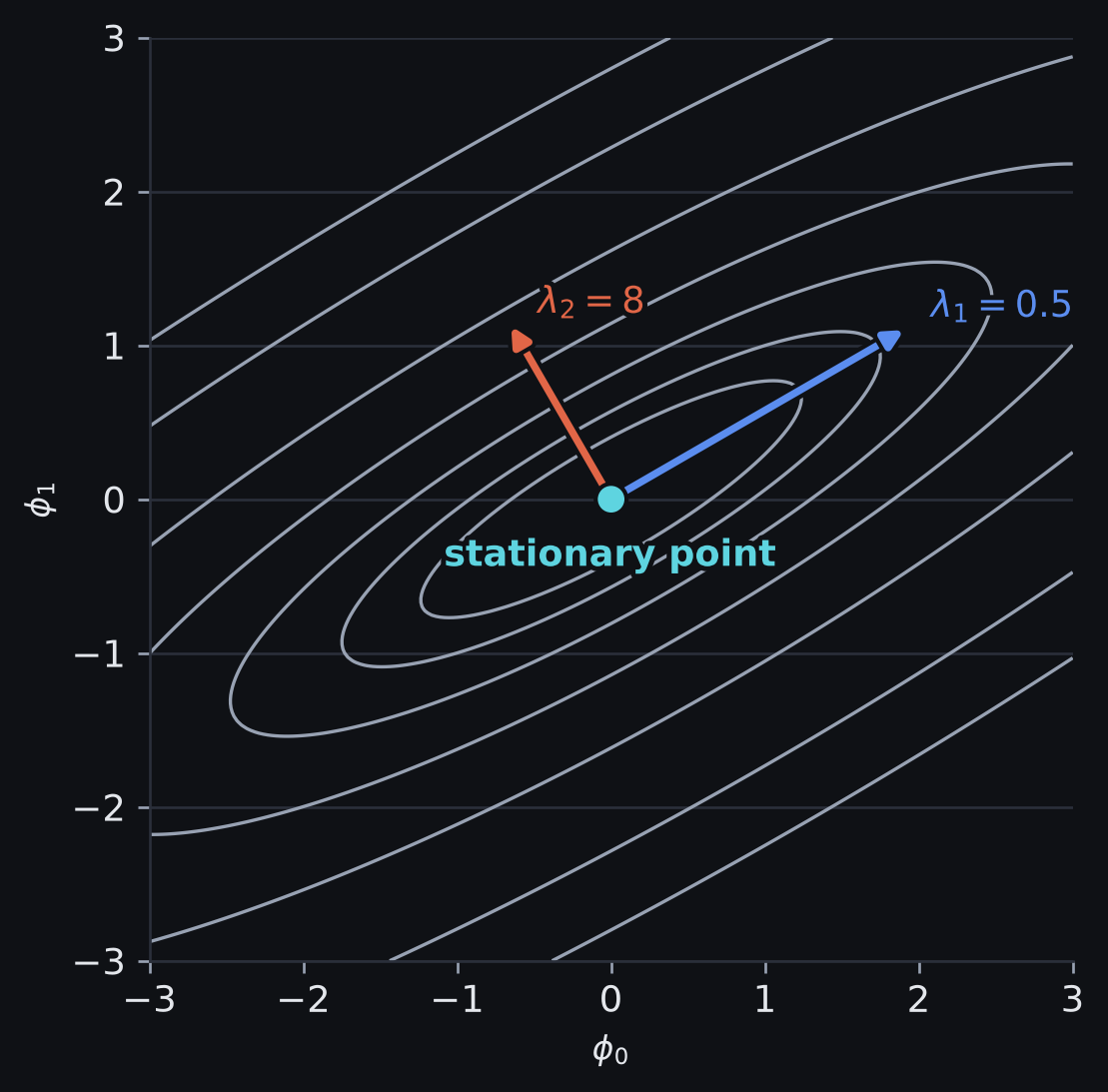
The Hessian eigenvectors give the principal curvature directions. One direction can be shallow while another is steep, producing an elongated valley.

• The long arrow marks the shallow direction; the valley runs along it
• The short arrow marks the steep direction across the valley
• Arrow length is for legibility; the printed eigenvalue is the curvature

Hessian geometry

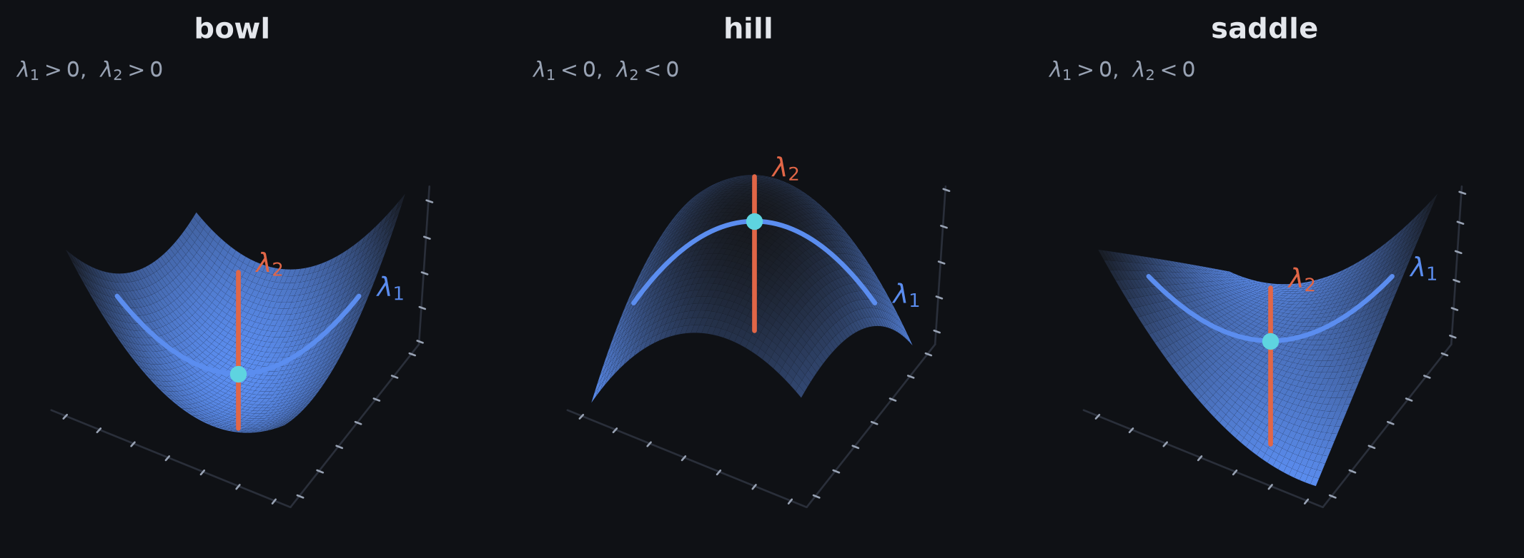
The signs of the Hessian eigenvalues distinguish locally bowl-shaped, hill-shaped, and saddle-like geometry.

• Connect eigenvalue signs to local shape
• Mixed-sign curvature means there are both locally uphill and downhill directions

Classifying stationary points

At a stationary point where \(\nabla_{\params}\loss=\vect{0}\):

• all eigenvalues \(>0\) → locally bowl-shaped → strict local minimum
• all eigenvalues \(<0\) → locally hill-shaped → strict local maximum
• mixed signs → some directions up, some down → saddle point

Zero eigenvalues require more care: second-order information alone may not decide the case.

Convexity and the Hessian

For a twice-differentiable function on a convex domain:

• positive semidefinite, \(\mat{H}\succeq 0\): every eigenvalue is non-negative, so no direction curves downward
• \(\mat{H}(\params)\succeq 0\) everywhere is sufficient for convexity
• \(\mat{H}(\params)\succ 0\) everywhere gives strict convexity

Non-convex neural-network losses

For models nonlinear in their parameters, the loss landscape is generally non-convex.

• adding nonlinear input features such as \(x^2\) does not destroy convexity if the model remains linear in \(\params\)
• placing parameters inside nonlinear functions can produce a non-convex loss surface

Non-convex landscape features

Possible features include:

• many valleys
• local minima
• saddle points
• long flat directions
• directions with very different curvature

The gradient still gives a local descent direction, but non-convexity removes the guarantee that following it will reach the global minimum.

Non-convex does not mean untrainable

Non-convexity removes the global-minimum guarantee. It does not imply that gradient-based training fails.

The Gabor model

Prince’s Gabor model (equation 6.8):

\[ \model{x} = \sin(z)\,\exp\!\left(-\frac{z^{2}}{32}\right), \qquad z=\phi_0+0.06\,\phi_1x. \]

• \(\phi_0\) shifts the wave along the input axis
• \(\phi_1\) squeezes or stretches it
• The data: 40 noisy samples from one true setting of the pair

With two parameters we can still plot the complete loss surface; unlike least squares, it is non-convex.

Convex and non-convex loss landscapes

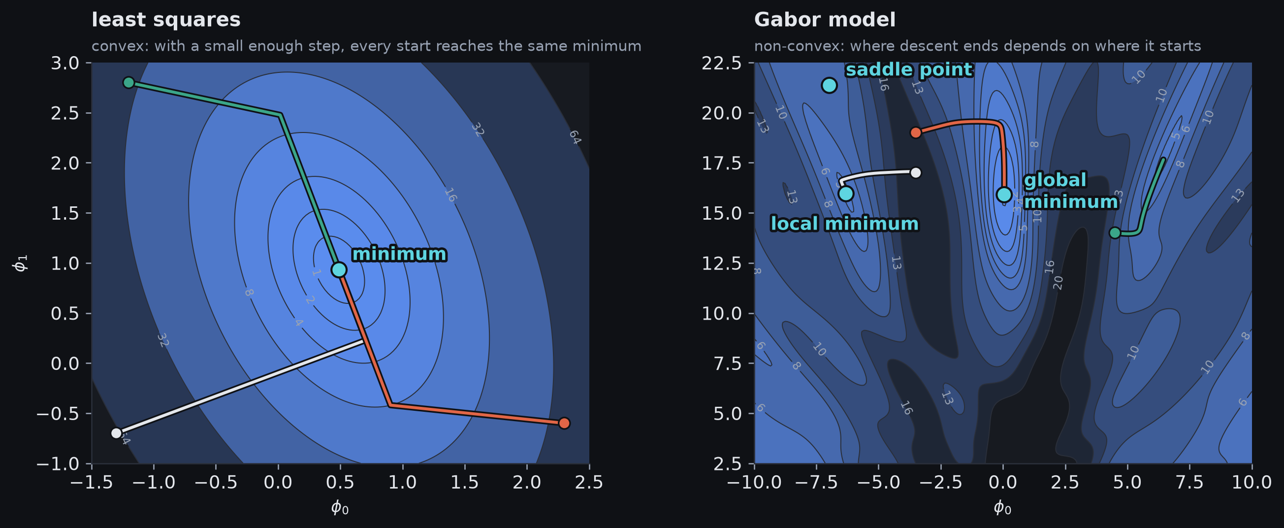
Convex objectives have no suboptimal local minima; non-convex objectives can contain multiple valleys and saddle points.

• Same descent rule, different geometry: the global-minimum guarantee is gone
• Compare where identical update rules finish from different starting points

Local minima and saddle points

A local minimum has no nearby downhill direction, but a better solution may exist elsewhere.

A saddle point need not be a minimum even when the gradient is zero. At a strict saddle, curvature is upward in some directions and downward in others.

Therefore

\[ \nabla_{\params}\loss\approx \vect{0} \]

shows that the local slope is small; it does not prove that the global minimum has been found.

Second-order methods

Near a well-behaved local minimum, second-order methods such as Newton’s method use curvature to rescale the gradient:

\[ \Delta\params \approx -\mat{H}\inv\nabla_{\params}\loss. \]

Curvature adjusts the scale of the update:

• steep curvature → move cautiously
• shallow curvature → move further

But a neural network with millions of parameters would have an enormous Hessian. Forming and inverting it directly is usually impractical.

Stochastic and adaptive optimisation

Cost of full-batch updates

The full gradient uses every training example:

\[ \nabla_{\params}\loss = \sum_{i=1}^{I}\nabla_{\params}\exloss_i. \]

For a large dataset, computing that exact sum before every update is expensive. A minibatch lets us update the parameters after examining only part of the dataset.

Stochastic gradient descent

Instead of using the whole dataset, choose a minibatch \(\set{B}_t\) at step \(t\).

Define the minibatch gradient

\[ \vect{g}_t = \frac{1}{|\set{B}_t|} \sum_{i\in \set{B}_t} \nabla_{\params}\exloss_i(\params_t). \]

Then update

\[ \params_{t+1} = \params_t - \alpha\vect{g}_t. \]

Averaging makes the gradient scale less dependent on batch size. Relative to the earlier sum-loss convention, this estimates \(\frac{1}{I}\nabla_{\params}\loss\); the constant factor \(I\) can be absorbed into the learning rate.

Minibatch gradient variation

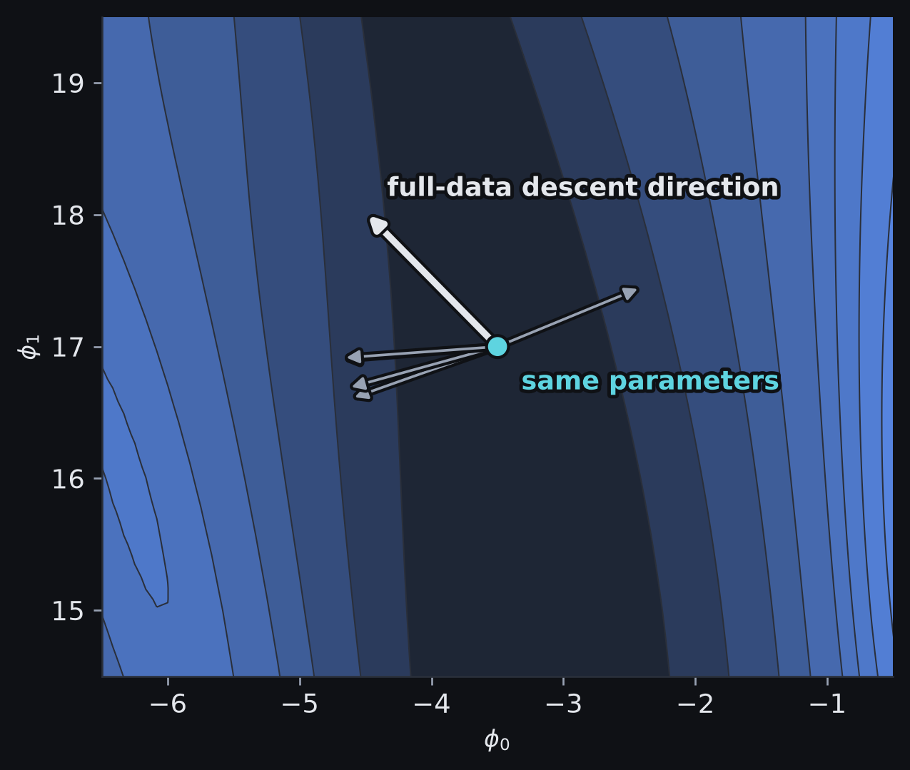
At the same parameter setting, different minibatches give different descent directions. The highlighted arrow is the full-data direction; all arrows are drawn at a fixed length, so only their direction carries meaning.

• Compare arrow directions only; lengths are normalised for display
• Each minibatch gives a different estimate of the full-data mean gradient
• Connect this directional variation to the stochastic trajectories

Full-batch and stochastic descent paths

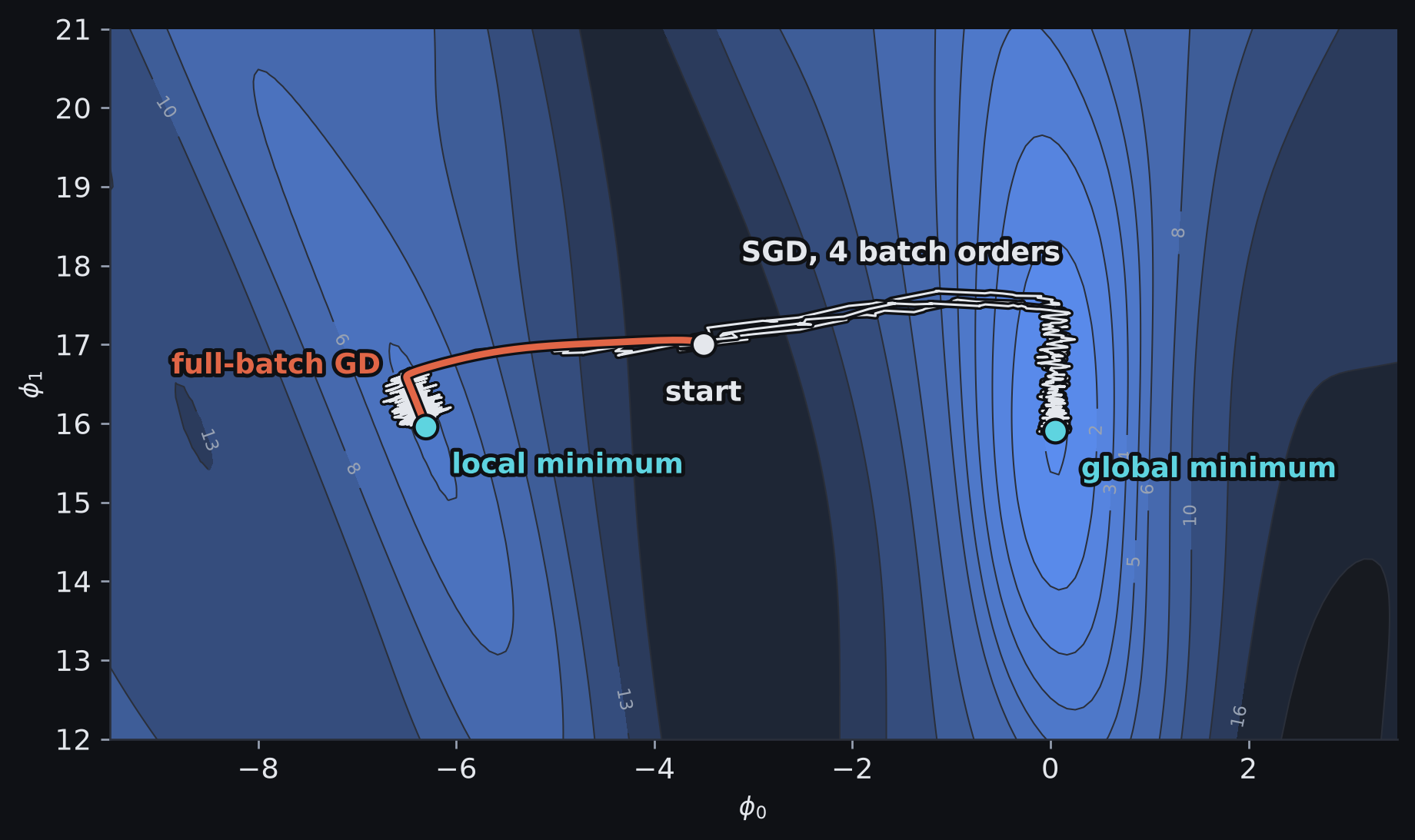
Full-batch gradient descent follows one deterministic gradient field; minibatch sampling perturbs the gradient and therefore the trajectory.

• Compare the deterministic full-data path with several minibatch trajectories
• Each minibatch supplies a different local gradient estimate at the same parameters

Effects of minibatching

A minibatch gradient is an estimate of the full-dataset mean gradient.

The sampling noise changes the optimisation trajectory.

Each batch defines a slightly different local estimate of “downhill.”

Minibatching introduces sampling noise into the trajectory:

• each step is cheaper
• updates begin before scanning the whole dataset
• the perturbed trajectory can sometimes move away from flat or suboptimal regions
• under uniform sampling, the expected minibatch gradient equals the full-dataset mean gradient

Batch size and learning rate interact

Batch size and learning rate jointly determine how noisy the parameter trajectory is.

Batch, iteration, epoch

These terms describe different units of training.

• Batch / minibatch: the examples used to compute one gradient estimate
• Iteration / step: one parameter update
• Epoch: one pass through the training dataset

Special cases:

• batch size \(1\) → classical stochastic update
• batch size = dataset size → full-batch gradient descent

Shuffling without replacement

A common training loop shuffles the examples and then forms minibatches without replacement.

This ensures that:

• within an epoch, each training example contributes once
• between steps, the optimiser sees different subsets and therefore different gradient estimates

The randomness comes from which examples are grouped together and when they are seen.

Stochastic trajectories

With full-batch gradient descent, each point in parameter space has one deterministic gradient.

With SGD, the gradient also depends on the sampled batch:

\[ \vect{g}_t = \vect{g}(\params_t,\set{B}_t). \]

SGD therefore follows the gradient of a slightly different minibatch loss at each step.

The path may temporarily move uphill on the full training loss even when the current minibatch gradient points downhill for its own batch.

Learning-rate schedules

Many training schedules use larger steps early and reduce them later.

Early training:

• parameters may still be far from a low-loss region
• larger steps can move through parameter space quickly

Later training:

• parameters may be nearer a low-loss region
• smaller steps allow finer adjustment

A learning-rate schedule reduces \(\alpha\) during training.

Some training recipes also use warm-up: begin with a very small learning rate and gradually increase it, limiting early update sizes while activations, gradients, and optimiser state may not yet be well behaved.

Oscillation in narrow valleys

Imagine a long narrow valley:

• very steep from side to side
• shallow along its length

Plain gradient descent can zig-zag across the steep direction while making slow progress along the shallow direction.

Momentum averages gradients over successive steps: persistent directions reinforce, while directions that keep reversing tend to cancel.

Momentum

Let \(\vect{g}_t\) be the current minibatch gradient.

Momentum maintains an exponentially smoothed gradient:

\[ \underbrace{\vect{m}_{t+1}}_{\text{smoothed gradient}} = \underbrace{\beta\vect{m}_t}_{\text{keep some history}} + \underbrace{(1-\beta)\vect{g}_t}_{\text{add current evidence}}. \]

Then update

\[ \params_{t+1} = \params_t - \alpha\vect{m}_{t+1}. \]

Under a constant gradient, this exponential moving average settles at \(\vect{m}=\vect{g}\).

Momentum in a narrow valley

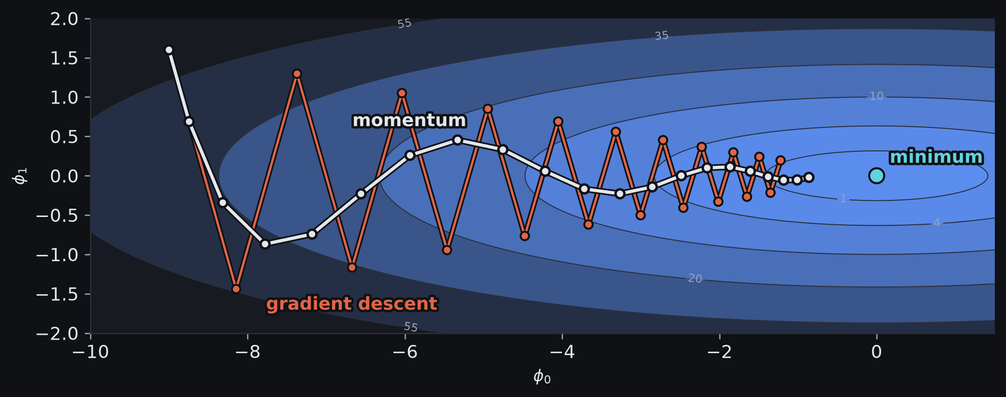
Averaging gradients over time damps oscillation across steep directions while preserving progress along persistent directions.

• Point out cancellation across the steep direction and reinforcement along the valley
• Connect the cancellation picture to the moving-average formula
• The deck uses the EMA convention with \((1-\beta)\); some libraries parameterise momentum differently, so compare formulas rather than raw coefficient values

Persistent and reversing gradients

Repeatedly aligned gradients reinforce one another.

Repeatedly reversing gradients cancel one another.

Momentum tends to:

• reinforce persistent directions
• damp oscillation in reversing directions
• smooth minibatch noise

\(\beta\) controls memory:

• small \(\beta\) → react strongly to the current batch
• large \(\beta\) → average over a longer history

Nesterov momentum

Ordinary momentum measures the gradient where we are now and then combines it with momentum.

Nesterov momentum first moves to the position predicted by the momentum term.

\[ \text{look-ahead point} = \params_t - \alpha\beta\vect{m}_t. \]

Then measure the gradient at that predicted position.

The gradient at the look-ahead point corrects the momentum-predicted trajectory.

The Nesterov look-ahead

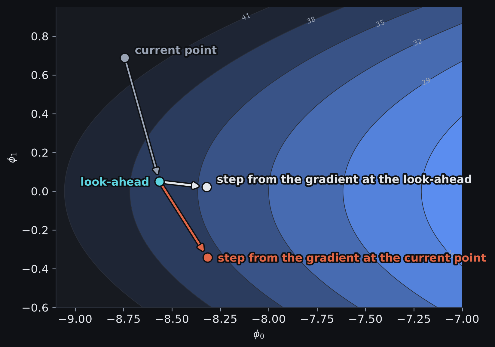
Nesterov momentum first follows the momentum direction, then evaluates the gradient at the predicted look-ahead point.

• Contrast the gradient evaluation point for ordinary and Nesterov momentum
• Emphasise the gradient as a correction at the look-ahead point

Coordinatewise step scales

A fixed global learning rate assumes the same step scale is sensible in every coordinate.

• Gradient magnitudes differ across layers and parameters, often by orders of magnitude
• one global \(\alpha\) is then too large in some coordinates and too small in others

Adaptive methods instead scale each coordinate using its own gradient history.

• coordinatewise scaling can compensate for different gradient magnitudes across coordinates
• it cannot rotate the coordinate system to align with an oblique steep direction

AdaGrad introduced this general idea; RMSProp and AdaDelta modified how squared-gradient history is accumulated. Adam combines this adaptive scaling with momentum-like averaging of the gradient itself.

Coordinatewise gradient scaling

Suppose the gradient is \(\vect{g}_t\).

As a thought experiment, divide each coordinate by its own magnitude:

\[ \frac{\vect{g}_t}{\sqrt{\vect{g}_t\odot\vect{g}_t}+\epsilon}, \]

then for \(|g_{t,j}|\gg\epsilon\), each coordinate is approximately \(\operatorname{sign}(g_{t,j})\).

This is coordinatewise scaling, not vector normalisation by \(\lVert\vect{g}_t\rVert\).

• \(\odot\) means elementwise multiplication
• \(\epsilon\) prevents division by zero

This prevents steep coordinates from automatically receiving the largest parameter changes, but using only the sign discards too much information and can oscillate around the minimum.

Adam: direction and scale

Adam maintains two moving averages.

First moment — a smoothed gradient:

\[ \vect{m}_{t+1} = \beta_1\vect{m}_t + (1-\beta_1)\vect{g}_t. \]

Second raw moment — a smoothed squared gradient:

\[ \vect{v}_{t+1} = \beta_2\vect{v}_t + (1-\beta_2) (\vect{g}_t\odot\vect{g}_t). \]

\(\vect{m}_t\) tracks the recent signed gradient; \(\vect{v}_t\) tracks typical squared magnitude per coordinate.

The terminology “first moment” and “second raw moment” is mean-like language. In particular, \(\vect{v}_t\) is not the variance of the gradient.

In PyTorch, Adam(betas=...) takes the pair \((\beta_1, \beta_2)\).

Adam’s two moving averages

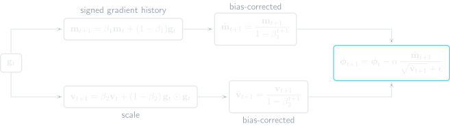
Adam combines a moving average of gradients with a moving average of squared gradients to produce an adaptively scaled update.

• Label \(\vect{m}_t\) as direction history and \(\vect{v}_t\) as coordinatewise scale history
• Read the diagram left to right before showing the compact update equation

Adam bias correction

At the start of training,

\[ \vect{m}_0=\vect{0}, \qquad \vect{v}_0=\vect{0}. \]

Because both moving averages start at zero, their early values are biased toward zero.

Adam compensates with

\[ \tilde{\vect{m}}_{t+1} = \frac{\vect{m}_{t+1}}{1-\beta_1^{t+1}}, \qquad \tilde{\vect{v}}_{t+1} = \frac{\vect{v}_{t+1}}{1-\beta_2^{t+1}}. \]

As \(t\) grows, \(\beta_1^{t+1}\) and \(\beta_2^{t+1}\) shrink and the bias-correction factors approach one.

The Adam update

The parameter update is

\[ \params_{t+1} = \params_t - \underbrace{\alpha}_{\text{global scale}} \frac{ \underbrace{\tilde{\vect{m}}_{t+1}}_{\text{smoothed gradient}} }{ \underbrace{\sqrt{\tilde{\vect{v}}_{t+1}}}_{\text{coordinatewise scale}} + \underbrace{\epsilon}_{\text{numerical stability}} }. \]

Adam combines momentum-like gradient smoothing with per-coordinate adaptive scaling. The square root and division are applied elementwise.

Effect of adaptive scaling

A single global step size is difficult to tune when gradient magnitudes differ substantially across coordinates.

Adam reduces the effective step in coordinates with persistently large squared gradients and allows relatively larger movement where gradients have been smaller.

Adaptive scaling reduces sensitivity to differences in gradient scale across coordinates, but the global learning rate still matters.

Adam versus SGD

The relative behaviour of adaptive methods and SGD depends on the objective and training setup.

In practice:

• Adam often makes rapid initial progress
• SGD with momentum can be highly competitive when carefully tuned
• optimiser comparisons are entangled with learning-rate schedules and other hyperparameters

Neither optimiser dominates across architectures, datasets, and training recipes.

Optimisers and backpropagation

Parameters vs hyperparameters

Model parameters are learned from data:

\[ \params. \]

Training hyperparameters control the learning procedure, for example:

• optimiser choice
• learning rate and schedule
• batch size
• momentum coefficients
• number of epochs

Parameters are optimised inside one training run.

Hyperparameters are compared across training runs.

Information used by each optimiser

The optimisers differ in the information used to construct each update.

Gradient descent

• current gradient

Momentum

• current gradient + recent gradient history

Adam

• smoothed gradient history + coordinatewise squared-gradient history

Newton-style methods

• current gradient + explicit Hessian curvature

Where the optimiser acts

Training repeatedly follows this sequence:

\[ \text{parameters} \rightarrow \text{predictions} \rightarrow \text{loss} \rightarrow \text{gradient} \rightarrow \text{parameter update}. \]

Once the gradient is known, the optimisation methods in this lecture perform the final step:

\[ \nabla_{\params}\loss \quad\longrightarrow\quad \Delta\params. \]

The optimiser decides how to turn that gradient into a parameter update.

For a deep network, the remaining problem is to compute that gradient efficiently.

Deep networks as function compositions

A deep network does not map parameters to loss in one step.

A simplified computation looks like

\[ \vect{x} \rightarrow \hidden_1 \rightarrow \hidden_2 \rightarrow \cdots \rightarrow \hat{\vect{y}} \rightarrow \loss. \]

Each intermediate quantity depends on the one before it, so changing an early parameter can affect the loss through many successive operations.

The chain rule tells us how to compose these local sensitivities.

Computation graph: forward and backward

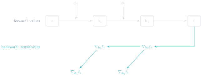
The forward computation produces activations and a loss; the reverse computation asks how that loss is sensitive to earlier quantities and parameters.

• Reuse the language of sensitivities from earlier in the lecture
• Ask what quantities the optimiser ultimately needs: gradients with respect to each parameter block
• Stop at the computational problem; do not derive the reverse-mode algorithm here

The gradient problem in deep networks

Suppose the network is written as a composition

\[ \hidden_1=\vmodel[\params_1]{\vect{x}}, \qquad \hidden_2=\vmodel[\params_2]{\hidden_1}, \qquad \exloss_i=\exloss(\hidden_2). \]

• One example at a time here: dataset or minibatch gradients aggregate these per-example gradients

The optimiser ultimately needs sensitivities such as

\[ \nabla_{\params_1}\exloss_i, \qquad \nabla_{\params_2}\exloss_i. \]

Computing those gradients independently, parameter by parameter, would be impractical in a deep network.

Backpropagation is the efficient reverse computation used to obtain them from the computation graph.

Initialisation affects gradient scale

Backpropagation repeatedly combines derivatives from successive layers.

For an early layer, the gradient contains products of many local derivative terms.

If those terms are repeatedly small, the gradient can shrink as it moves backward.

If they are repeatedly large, the gradient can grow rapidly.

The initial parameter values therefore affect not only the initial predictions, but also the scale of the gradients available for learning.

Two issues become central in deep networks:

• gradient computation: obtain all parameter sensitivities efficiently
• initialisation: choose starting parameters that preserve useful signal and gradient scales

Backpropagation addresses the first; the choice of initial parameter distribution addresses the second.

Summary

• Training is optimisation in parameter space
• A partial derivative measures sensitivity to one parameter; \(\nabla_{\params}\loss\) stacks all parameter sensitivities into the gradient
• Gradient descent uses the locally steepest first-order downhill direction
• The Jacobian organises first derivatives of vector-valued functions
• The Hessian organises second derivatives; its eigenvectors give principal curvature directions and its eigenvalues give signed curvature
• Non-convex losses can contain multiple minima, saddle points, and flat directions
• Minibatches trade exact gradients for cheaper, noisy estimates
• Momentum smooths gradient history; Adam also rescales coordinates adaptively
• Deep networks require efficient computation of parameter gradients; backpropagation addresses that problem

Source and reading

Primary source for this lecture:

• Simon J. D. Prince, Understanding Deep Learning, Chapter 6, Fitting Models
• Appendix B.5 for the matrix-calculus notation used in the gradient and Hessian sections