Lecture 3: Loss Functions

Block 4.2 Advanced AI

Eoin O’Brien

Where we are

Linear regression, shallow neural networks, and deep neural networks define families of functions
The parameters \(\params\) select one member of that family
An architecture tells us what mappings are possible
Training still needs a criterion for deciding which mapping is best

\[ \text{model family} \quad \model{\vect{x}} \qquad\Longrightarrow\qquad \text{training criterion} \quad \loss[\params] \]

We will construct that criterion from probabilistic modelling assumptions

Learning objectives

By the end of this lecture, you should be able to:

explain how loss functions define what it means for a model to fit the data well
interpret neural networks as predicting parameters of probability distributions, not only point estimates
distinguish probability mass, probability density, conditional probability, and likelihood
construct and interpret likelihood, log-likelihood, and negative log-likelihood
explain why logarithms turn likelihood products into sums without changing the optimum

Learning objectives (cont.)

derive least squares from a Gaussian model and distinguish homoscedastic from heteroscedastic regression
derive binary and multiclass cross-entropy from Bernoulli and categorical models
construct likelihood-based losses for multiple outputs and state the required independence assumptions
use expectation, cross-entropy, and KL divergence to connect maximum likelihood, NLL, and empirical cross-entropy

Training data and loss

Assume a training dataset

\[ \set{D}=\{(\vect{x}_i,y_i)\}_{i=1}^{I}. \]

\(\vect{x}_i\) — the \(i\)th input
\(y_i\) — its ground-truth target
\(I\) — number of training examples

A loss function assigns a scalar score to a parameter setting:

\[ \loss[\params]\in\reals, \qquad \hat{\params} = \argmin_{\params} \loss[\params]. \]

Lower loss means better agreement with the chosen training criterion

What does \(\argmin\) return?

A loss function scores every candidate parameter setting. Training wants the parameter value at the bottom of the loss landscape.

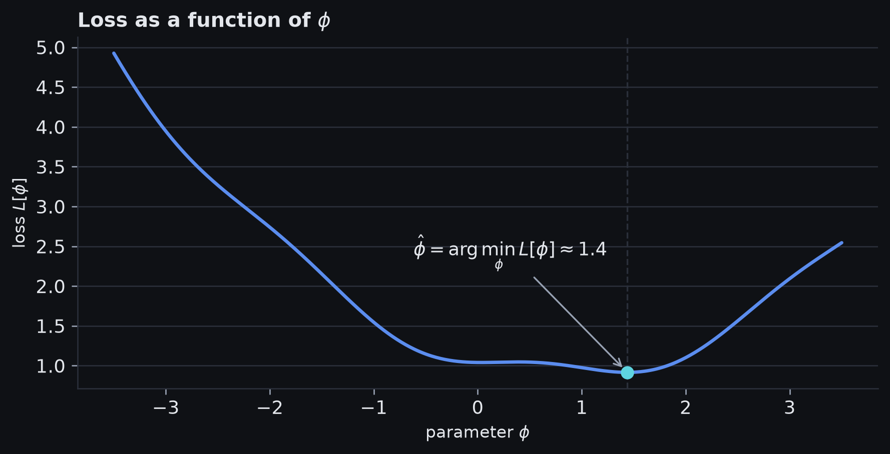
A one-dimensional loss landscape. \(\hat{\phi}\) is the parameter value at the minimum.

\(\min_{\params}\loss[\params]\) is the lowest loss value
\(\argmin_{\params}\loss[\params]\) is the parameter setting that achieves it
training returns the second object: \(\hat{\params}\)

Reminder: least squares

For real-valued regression, a familiar choice is

\[ \loss[\params] = \sum_{i=1}^{I} \left(y_i-\model{\vect{x}_i}\right)^2. \]

Each residual measures the prediction error
Squaring removes the sign and penalises larger deviations more strongly
But least squares is not appropriate for every kind of target

Question: why this loss — and what should we use for other output types?

Different outputs need different models of uncertainty

Task	Output domain	Example
Regression	\(y\in\reals\)	temperature
Binary classification	\(y\in\{0,1\}\)	spam / not spam
Multiclass classification	\(y\in\{1,\ldots,K\}\)	object category
Count prediction	\(y\in\{0,1,2,\ldots\}\)	number of arrivals
Direction	\(y\in(-\pi,\pi]\)	orientation angle

The target domain constrains which probability distributions are sensible
Our modelling assumptions choose a distribution within those constraints
That choice will determine the corresponding maximum-likelihood loss

Maximum likelihood

What does a point prediction leave out?

Suppose two weather models both predict

\[ \hat y = 20^\circ\mathrm{C}. \]

The same point estimate can still represent very different uncertainty:

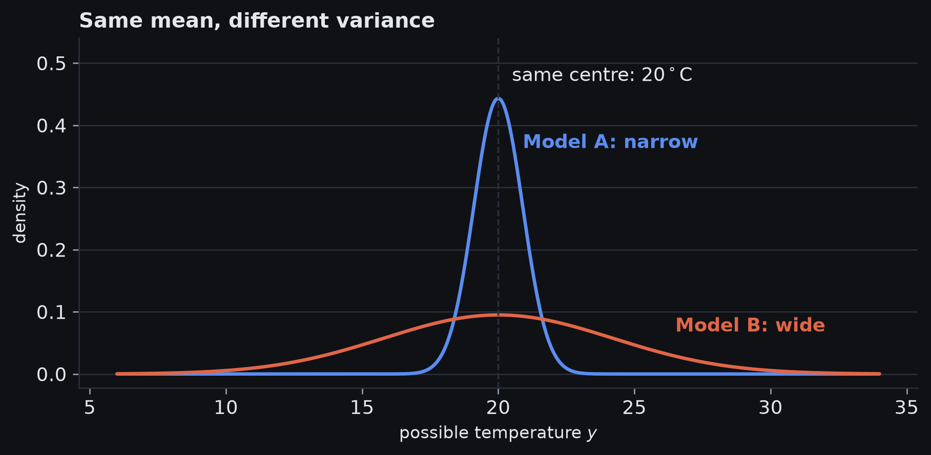
Two Gaussian predictive distributions with mean \(20^\circ\mathrm{C}\) and different variances.

\[ \boxed{\text{same point estimate} \;\not\Rightarrow\; \text{same uncertainty}} \]

A point estimate tells us where to predict
A predictive distribution also tells us which other outcomes remain plausible

From one number to a predictive distribution

A point-prediction view returns one number:

\[ \hat y=\model{\vect{x}}. \]

A probabilistic view returns the parameters of a distribution:

\[ \distparams =\model{\vect{x}}, \qquad y\sim p(y\mid\distparams). \]

the network still computes a deterministic function of \(\vect{x}\)
its output now tells us which predictive distribution to use
a point estimate can still be extracted from that distribution at inference time

The network remains deterministic; its output parameterises a predictive distribution over \(y\).

From input to predictive distribution

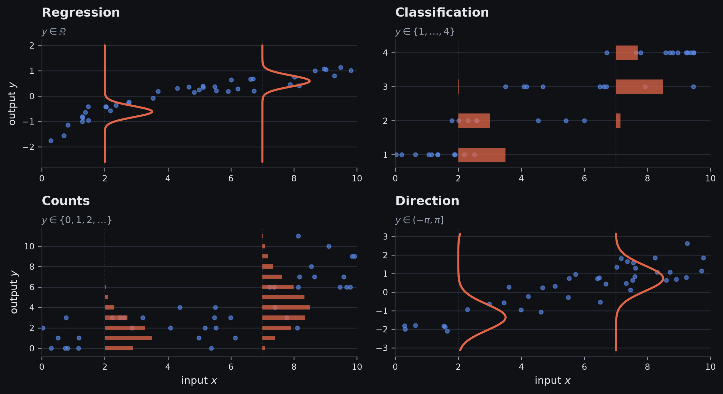
Predictive distributions at two input values for regression, classification, count, and directional targets.

The network does not need to output a whole probability curve or table directly
It predicts the parameter(s) \(\distparams\) of a chosen distribution family
The same construction applies in all four panels; the distribution family and parameterisation change.

A distribution is a family with knobs

A probability distribution is not an arbitrary curve the network must draw from scratch.

Choose a distribution family, then let its parameters act as adjustable knobs:

Distribution	Parameters	What the parameters control
Normal	\(\mu,\sigma^2\)	centre and spread
Bernoulli	\(\lambda\)	probability of class \(1\)
Categorical	\(\lambda_1,\ldots,\lambda_K\)	probability allocated to each class

A distribution is a family with knobs (cont.)

In general,

\[ p(y\mid\distparams), \qquad \distparams_i=\model{\vect{x}_i}. \]

we choose the family from the prediction problem
the network predicts the knob settings for each input
the loss will follow from how much probability or density that distribution assigns to the observed target

Probability is a budget of 1

Think of a distribution as having one unit of probability to allocate.

Discrete outcomes: split that unit among separate possibilities.

\[ \sum_y p(y)=1. \]

A bar height is itself a probability.

Continuous outcomes: spread that unit across a continuum.

\[ \int p(y)\,dy=1. \]

Probability is now an area under the density curve, not the height at one point.

A narrow density can rise above \(1\) without violating probability rules; its total area is still \(1\).

A density can be greater than \(1\)

Consider a continuous variable that is uniform on the interval \([0,0.5]\).

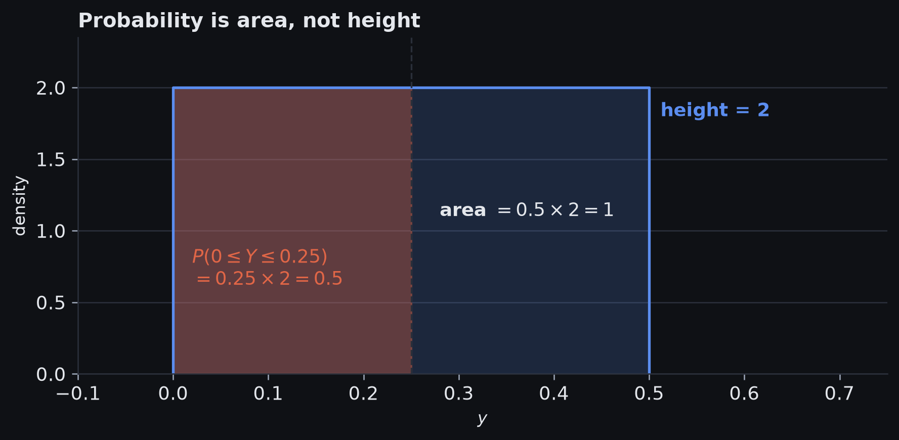
Uniform density on \([0,0.5]\): height \(2\), width \(0.5\), total area \(1\).

the density height is \(2\), which is perfectly valid
the area over the whole support is \(1\)
probabilities of intervals are obtained by taking areas

Probability mass and probability density

A random variable represents a quantity whose value is uncertain. Its distribution describes which values are plausible and how strongly they are weighted.

Discrete random variable

\(p(y)\) is a probability mass function
\(0\le p(y)\le1\)
masses over all possible values sum to \(1\)

Probability mass and probability density (cont.)

Continuous random variable

\(p(y)\) is a probability density function
an exact point has probability \(0\)
density is non-negative and may exceed \(1\)
probability over an interval is the area under the density on that interval

Maximum likelihood scores an observed discrete value by its probability mass and an observed continuous value by its density.

Reading \(p(y_i\mid f[\vect{x}_i,\params])\) in words

For one training example, we will repeatedly write

\[ p\!\left(y_i\mid \model{\vect{x}_i}\right). \]

Read it from the inside out:

\(\vect{x}_i\) is the observed input for example \(i\).
\(\model{\vect{x}_i}\) is the network output for that input, interpreted as parameter(s) of the chosen predictive distribution.
\(p(y\mid\model{\vect{x}_i})\) is the resulting distribution over possible target values \(y\).
Set \(y=y_i\): evaluate that distribution at the target that was actually observed.

In words: given input \(\vect{x}_i\) and the current network parameters \(\params\), how much probability mass or density does the resulting predictive distribution assign to the observed target \(y_i\)?

Reading \(p(y_i\mid f[\vect{x}_i,\params])\) in words (cont.)

Equivalently, using \(\distparams_i=\model{\vect{x}_i}\),

\[ \vect{x}_i \longrightarrow \distparams_i \longrightarrow p(y\mid\distparams_i) \longrightarrow p(y_i\mid\distparams_i). \]

for a discrete target, this is probability mass
for a continuous target, this is probability density
the notation is schematic: the network may predict a mean, a probability, logits that are transformed into probabilities, or several distribution parameters; fixed parameters may be omitted

Expectation is a probability-weighted average

Suppose

\[ P(Y=0)=0.2, \qquad P(Y=1)=0.5, \qquad P(Y=2)=0.3. \]

The expected value is

\[ \expect{Y} = 0(0.2)+1(0.5)+2(0.3) = 1.1. \]

common outcomes count more heavily than rare outcomes
the expectation itself need not be a possible outcome

Expectation means “average according to this distribution.”

Expectation in general

For a function \(g(Y)\), expectation averages the value of \(g\) using the probabilities of \(Y\) as weights.

Discrete: \[ \expectsub{Y\sim q}{g(Y)} = \sum_y g(y)q(y). \]

Continuous: \[ \expectsub{Y\sim q}{g(Y)} = \int g(y)q(y)\,dy. \]

\(g(Y)=Y\) gives the mean
\(g(Y)=(Y-\mu)^2\) gives the variance when averaged

From one observation to many

For one training pair \((\vect{x}_i,y_i)\), define the model score for what actually happened:

\[ p_i = p\!\left(y_i\mid \model{\vect{x}_i}\right). \]

a good model assigns high mass or density to the observed target
a dataset contains many such observations
we therefore need a rule for combining the per-example terms

The rule will come from an independence assumption.

Why independent probabilities multiply

Start with two independent fair coin tosses.

\[ P(H,H) = P(H)P(H) = \frac12\times\frac12 = \frac14. \]

Why multiply?

the first factor says how plausible the first event is
the second says how plausible the second event is
the joint event requires both to occur

For independent variables in general,

\[ p(a,b)=p(a)p(b). \]

Conditional independence in supervised learning

For all training targets together, the model concerns the joint distribution

\[ p(y_1,\ldots,y_I\mid\vect{x}_1,\ldots,\vect{x}_I). \]

The standard supervised-learning model assumes the targets are conditionally independent once their inputs are given:

\[ p(y_1,\ldots,y_I\mid\vect{x}_1,\ldots,\vect{x}_I) = \prod_{i=1}^{I}p(y_i\mid\vect{x}_i). \]

Conditional independence in supervised learning (cont.)

each target is modelled from its corresponding input
observations share the same form of predictive distribution, while its parameters may vary by input
dependence between training observations is ignored after conditioning on the inputs

This factorisation is a modelling assumption, not a property of neural networks.

Dataset likelihood

Apply the same factorisation to the per-example scores \(p_i\):

\[ \likelihood(\params;\set{D}) = \prod_{i=1}^{I}p_i = \prod_{i=1}^{I} p\!\left(y_i\mid \model{\vect{x}_i}\right). \]

Read the product as:

evaluate the model at every input \(\vect{x}_i\)
ask how much mass or density it assigns to the observed \(y_i\)
multiply those scores because the observations are conditionally independent

\(\likelihood\) is the likelihood function for the model parameters, with the observed dataset held fixed.

Conditional probability and likelihood

The vertical bar in

\[ p(y\mid\vect{x},\params) \]

is read “\(y\) given \(\vect{x}\) and \(\params\)”: it describes uncertainty in \(y\) once the conditioning quantities are fixed.

Conditional probability and likelihood (cont.)

The same expression has two roles.

Vary \(y\); fix \(\vect{x},\params\)

\(p(y\mid\vect{x},\params)\) is a probability mass function or density over possible outputs
it must normalise over \(y\)

Fix the observed \(y,\vect{x}\); vary \(\params\)

the same expression is a likelihood function of \(\params\)
it need not normalise over \(\params\)
likelihood is not a posterior probability over parameters

Density and likelihood

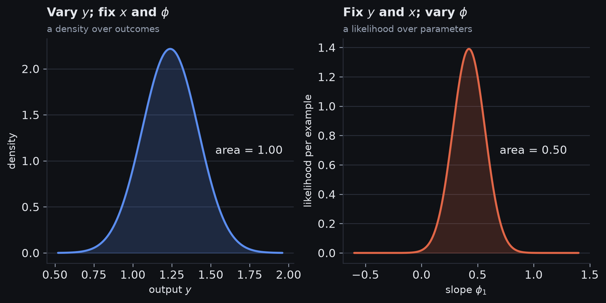
Fixing the parameters gives a density over outcomes; fixing the observation gives a likelihood as the parameter varies.

Left: a probability density. The area is \(1\), and it must be
Right: a likelihood. It need not integrate to \(1\) over the parameter
The likelihood curve is not a probability distribution over \(\phi_1\).

Maximum likelihood

Choose parameters that make the observed dataset as likely as possible:

\[ \hat{\params} = \argmax_{\params} \likelihood(\params;\set{D}) = \argmax_{\params} \prod_{i=1}^{I}p_i. \]

Equivalently,

\[ \hat{\params} = \argmax_{\params} \prod_{i=1}^{I} p\!\left(y_i\mid \model{\vect{x}_i}\right). \]

This is the maximum-likelihood criterion.

Why take logarithms?

Products of many small probability values can underflow numerically:

\[ 0.01\times0.02\times0.03\times\cdots \]

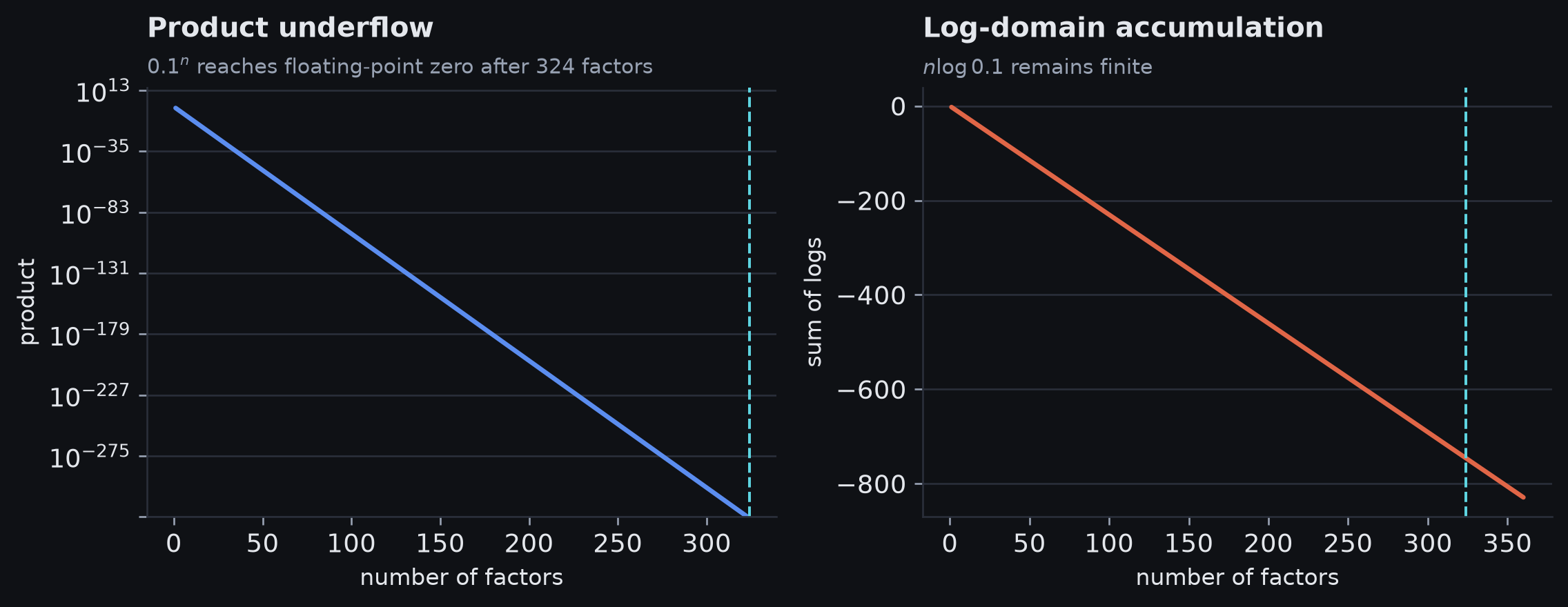
Product of repeated probability factors compared with the corresponding sum of log-probabilities.

A dataset of \(I\) examples multiplies \(I\) such factors together
Underflow is silent: the product becomes \(0\), and \(\log 0\) is \(-\infty\)

The logarithm solves this without changing which parameters are best.

Because \(\log\) is strictly increasing for positive arguments,

\[ a>b>0 \quad\Longleftrightarrow\quad \log a>\log b. \]

Therefore

\[ \argmax_{\params} \likelihood(\params;\set{D}) = \argmax_{\params} \log\likelihood(\params;\set{D}). \]

The logarithm and the argmax

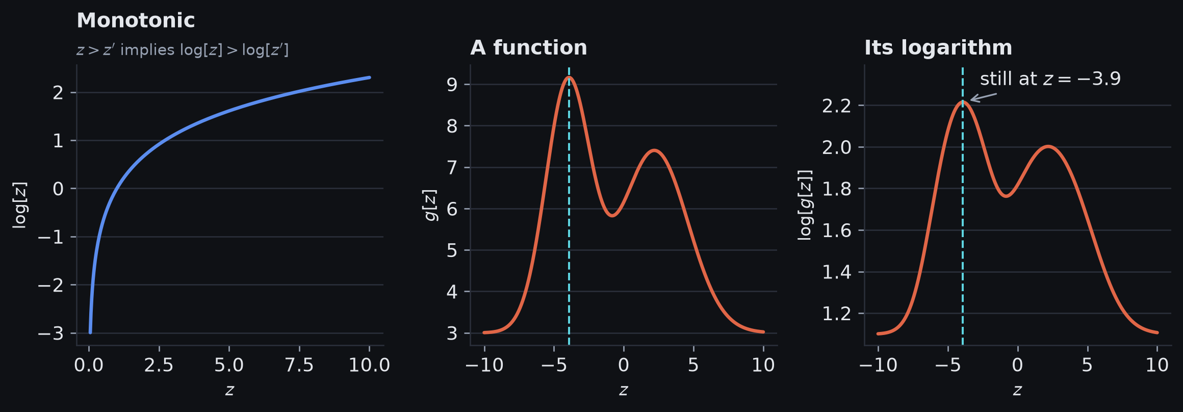
A positive function and its logarithm. The scale changes; the maximiser does not.

Strictly increasing transforms preserve ordering
The second peak is flattened, but it’s still the second peak
The logarithm changes the scale, but preserves the maximiser.

Likelihood becomes log-likelihood

Use the identity

\[ \log\!\left(\prod_i a_i\right) = \sum_i\log a_i. \]

Then

\[ \begin{aligned} \log\likelihood(\params;\set{D}) &= \log\!\left(\prod_{i=1}^{I}p_i\right)\\[4pt] &= \sum_{i=1}^{I}\log p_i\\[4pt] &= \sum_{i=1}^{I} \log p\!\left(y_i\mid \model{\vect{x}_i}\right). \end{aligned} \]

Likelihood becomes log-likelihood (cont.)

before the log, all examples must be plausible at once, so their scores multiply
after the log, each example contributes an additive log-score
the optimum is unchanged because the logarithm preserves ordering
sums are also easier to represent, differentiate, and compute stably

From likelihood to a loss

Training is conventionally written as a minimisation problem.

Maximising log-likelihood is equivalent to minimising its negative:

\[ \boxed{ \hat{\params} = \argmax_{\params}\likelihood = \argmax_{\params}\log\likelihood = \argmin_{\params}[-\log\likelihood] } \]

So define the negative log-likelihood:

\[ \loss[\params] = -\sum_{i=1}^{I} \log p\!\left(y_i\mid \model{\vect{x}_i}\right). \]

Per-example loss and dataset loss

Define one example’s contribution as

\[ \exloss_i(\params) = -\log p\!\left(y_i\mid \model{\vect{x}_i}\right). \]

Then

\[ \loss[\params] = \sum_{i=1}^{I}\exloss_i(\params). \]

Per-example loss and dataset loss (cont.)

Implementations often minimise the mean instead:

\[ \erisk[\params] = \frac{1}{I}\sum_{i=1}^{I}\exloss_i(\params). \]

For a fixed dataset and this objective alone, sum and mean have the same minimiser
If other terms such as regularisation are added, their relative scaling must be handled consistently

Negative log-likelihood measures surprise

For a discrete observed target with probability mass \(p\),

\[ \boxed{\exloss=-\log p} \]

This quantity is often read as surprise:

Probability assigned to what happened	Surprise \(-\log p\)
\(1\)	\(0\)
\(0.5\)	\(0.693\)
\(0.1\)	\(2.303\)
\(0.01\)	\(4.605\)

expected outcomes produce small loss
outcomes the model called almost impossible produce large loss

Negative log-likelihood measures surprise (cont.)

\[ \boxed{\text{training chooses parameters that make the observed data as unsurprising as possible}} \]

Continuous case: use probability density rather than mass. A density may exceed \(1\), so an individual continuous NLL contribution can be negative; the optimisation principle is unchanged.

Worked example: likelihood and NLL

Suppose two parameter settings assign these probabilities to the correct class labels:

	Example 1	Example 2	Example 3	Likelihood	NLL
Model A	\(0.8\)	\(0.7\)	\(0.6\)	\(0.336\)	\(\approx1.09\)
Model B	\(0.9\)	\(0.2\)	\(0.9\)	\(0.162\)	\(\approx1.82\)

\[ 0.336>0.162 \qquad\Longleftrightarrow\qquad 1.09<1.82. \]

Larger likelihood \(\Longleftrightarrow\) smaller NLL
Model B’s single probability of \(0.2\) substantially hurts the joint likelihood

Training and inference answer different questions

Training

Which \(\params\) make the observed dataset most likely?

\[ \hat{\params} = \argmin_{\params}\loss[\params]. \]

Inference

With \(\hat{\params}\) fixed, what should we report for a new input \(\vect{x}\)?

\[ p\!\left(y\mid \model[\hat{\params}]{\vect{x}}\right) \]

The predictive distribution is the model output in probabilistic form; a point estimate is an additional decision rule.

Point predictions from a predictive distribution

One common choice is the mode:

\[ \hat y_{\text{mode}} = \argmax_{y} p\!\left(y\mid \model[\hat{\params}]{\vect{x}}\right). \]

But the appropriate point estimate depends on what error or downstream decision matters:

mean: optimal under squared-error loss
median: optimal under absolute-error loss
mode: most probable / highest-density value

For a normal distribution these coincide:

\[ y\mid\vect{x}\sim\normal(\mu,\sigma^2) \quad\Longrightarrow\quad \text{mean}=\text{median}=\text{mode}=\mu. \]

Common misconceptions

“The network predicts a distribution, not a value.”
The network predicts distribution parameters; a decision rule can still produce a point estimate.

“Likelihood is the probability of the parameters.”
No. The observed data are fixed; likelihood scores candidate parameter settings.

“Taking logs changes the best parameters.”
No. A strictly increasing transform preserves their ordering and hence the optimum.

“NLL is just negative probability.”
No. It is the negative logarithm of the probability mass or density assigned to the observation.

Maximum likelihood summary

A loss turns “best model” into an optimisation problem
Maximum likelihood chooses parameters that make the observed targets plausible under a chosen statistical model
The network predicts distribution parameters \(\distparams_i=\model{\vect{x}_i}\)
Conditional-independence assumptions let the dataset likelihood factorise into per-example terms
Taking logs converts products to sums without changing the optimum
Negating the log-likelihood gives the standard minimisation loss

\[ \boxed{ \loss[\params] = -\sum_{i=1}^{I} \log p\!\left(y_i\mid \model{\vect{x}_i}\right) } \]

The target domain constrains sensible distributions; modelling assumptions choose one; its NLL becomes the loss

Recipe for constructing loss functions

Constructing a likelihood-based loss

For training data

\[ \set{D}=\{(\vect{x}_i,y_i)\}_{i=1}^{I}, \]

construct the loss as follows:

Choose a distribution \(p(y\mid\distparams)\) whose support matches the target domain.
Predict its parameter(s) with the model: \(\distparams=\model{\vect{x}}\).
Train by negative log-likelihood over the observed input/target pairs.
Infer by returning the predictive distribution, or a suitable point summary of it.

Steps 1–2 specify the statistical model; step 3 induces the training loss; step 4 specifies what is returned at prediction time.

The same construction across three tasks

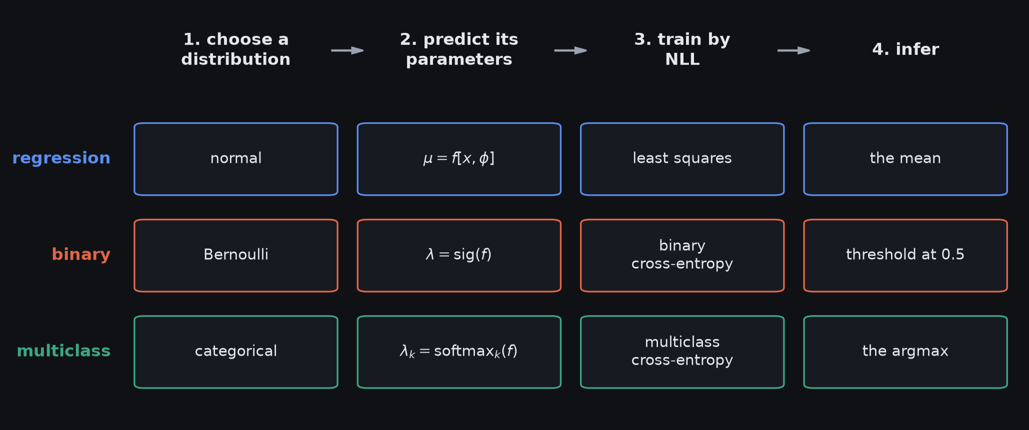
Four-step loss construction for regression, binary classification, and multiclass classification.

The columns are the recipe, and they never change
The rows are the three worked examples that follow, in the order we meet them
The distribution choice constrains the parameterisation and loss; inference depends on what the application needs returned.

The likelihood-based training objective

For each training example,

\[ \distparams_i=\model{\vect{x}_i}. \]

The computation for one example is

\[ \vect{x}_i \longrightarrow \distparams_i \longrightarrow p(y_i\mid\distparams_i) \longrightarrow -\log p(y_i\mid\distparams_i) \longrightarrow \exloss_i. \]

Sum those surprises over the dataset:

\[ \boxed{ \hat{\params} = \argmin_{\params} \left[ -\sum_{i=1}^{I} \log p\!\left(y_i\mid \model{\vect{x}_i}\right) \right] } \tag{5.6} \]

the pipeline stays the same across tasks
the chosen predictive distribution determines the concrete form of each \(-\log p\) term

What changes from task to task?

Modelling question	Task-specific choice
What values can \(y\) take?	the target domain
How should uncertainty over \(y\) be represented?	the distribution family \(p(y\mid\distparams)\)
What must the network output?	one or more parameters \(\distparams\)
What loss should be minimised?	the induced NLL \(-\log p(y\mid\distparams)\)
What should inference return?	the full distribution or an appropriate point summary

The domain constrains sensible distribution families; modelling assumptions choose among them.

Choosing a loss for a new task

For a new prediction problem, ask:

Domain: what kind of object is the target \(y\)?
Distribution: what \(p(y\mid\distparams)\) is defined on that domain and matches our assumptions?
Parameters: which components of \(\distparams\) should \(\model{\vect{x}}\) predict?
Loss: what does \(-\log p(y_i\mid\distparams_i)\) become for that distribution?
Inference: do we need the full predictive distribution or a point estimate?

The same questions apply across prediction problems; the distribution choice determines the resulting NLL.

Example 1: univariate regression

Apply the recipe: scalar regression

Goal: predict a single real-valued target

\[ y\in\reals \]

from an input \(\vect{x}\) using a model with parameters \(\params\).

Following the recipe:

choose a distribution defined on \(\reals\)
let the network predict its parameter(s)
minimise the resulting negative log-likelihood
use the fitted distribution for inference

For the first example, choose a univariate normal distribution.

Step 1: choose a normal distribution

Assume the target is distributed as

\[ y\mid\vect{x}\sim\normal(\mu,\sigma^2). \]

Its probability density is

\[ p(y\mid\mu,\sigma^2) = \frac{1}{\sqrt{2\pi\sigma^2}} \exp\!\left[ -\frac{(y-\mu)^2}{2\sigma^2} \right]. \tag{5.7} \]

\(\mu\in\reals\) controls the location of the distribution
\(\sigma^2>0\) controls its spread
\(\sigma=\sqrt{\sigma^2}\) is the standard deviation

Reading the Gaussian density

The Gaussian density can be read as two pieces:

\[ p(y\mid\mu,\sigma^2) = \underbrace{\frac{1}{\sqrt{2\pi\sigma^2}}}_{\text{normalises the total area}} \; \underbrace{\exp\!\left[-\frac12\left(\frac{y-\mu}{\sigma}\right)^2\right]}_{\text{downweights values far from }\mu}. \]

Step by step:

compute the distance from the centre: \(y-\mu\)
measure that distance in standard deviations: \((y-\mu)/\sigma\)
square it, so either direction counts equally
use the negative exponential so density falls rapidly with distance

At \(y=\mu\), the squared distance is \(0\) and the density is maximal.

Mean, variance, and the Gaussian parameters

For a random variable \(Y\), the mean is its expectation

\[ \mu=\expect{Y}, \]

and the variance is the expected squared deviation from that mean:

\[ \sigma^2 = \var{Y} = \expect{(Y-\mu)^2}. \]

For \(Y\sim\normal(\mu,\sigma^2)\):

\(\mu\) moves the centre of the bell curve left or right
\(\sigma=\sqrt{\sigma^2}\) is the standard deviation and controls its width
smaller \(\sigma^2\) gives a narrower, taller density; larger \(\sigma^2\) gives a broader density
mean = median = mode = \(\mu\)

Variance is average squared distance from the mean

Take four equally weighted observations with mean \(\mu=0\):

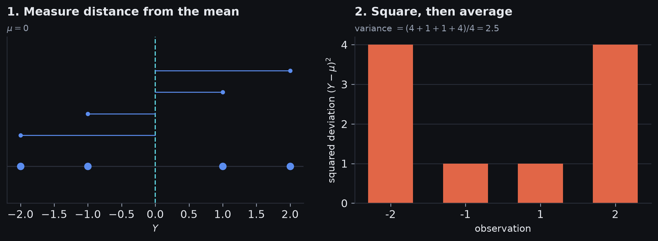
Distances from the mean and their squared values for four observations.

\[ \boxed{ \sigma^2 = \expect{(Y-\mu)^2} \;\approx\; \text{average squared distance from the mean} } \]

squaring removes the sign
larger deviations count more strongly
\(\sigma\) puts the spread back on the original units of \(Y\)

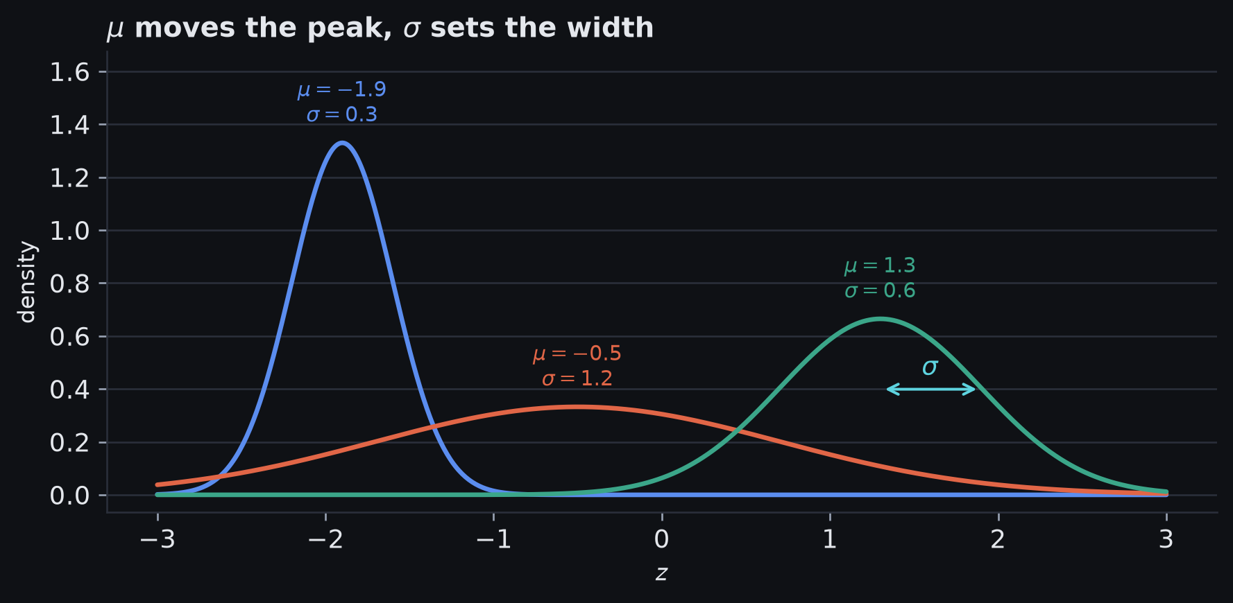
Normal distributions with different means and standard deviations.

The Gaussian therefore represents both a central prediction and uncertainty around it.

Step 2: predict the mean

Start with the simplest Gaussian regression model:

\[ \mu=\model{\vect{x}}, \]

while treating \(\sigma^2\) as a fixed constant.

Substituting the predicted mean into the normal density gives

\[ p\!\left(y\mid \model{\vect{x}},\sigma^2\right) = \frac{1}{\sqrt{2\pi\sigma^2}} \exp\!\left[ -\frac{\left(y-\model{\vect{x}}\right)^2}{2\sigma^2} \right]. \tag{5.8} \]

the network supplies the centre of the predictive distribution
every input currently shares the same assumed variance

Step 3: write the Gaussian NLL

For the training set \(\set{D}=\{(\vect{x}_i,y_i)\}_{i=1}^{I}\):

\[ \begin{aligned} \loss[\params] &= -\sum_{i=1}^{I} \log p\!\left(y_i\mid \model{\vect{x}_i},\sigma^2\right)\\[4pt] &= -\sum_{i=1}^{I} \log\!\left\{ \frac{1}{\sqrt{2\pi\sigma^2}} \exp\!\left[ -\frac{\left(y_i-\model{\vect{x}_i}\right)^2}{2\sigma^2} \right] \right\}. \end{aligned} \tag{5.9} \]

Training seeks \(\hat{\params}=\argmin_{\params}\loss[\params]\).

Reading the Gaussian NLL

After taking the negative logarithm, one example contributes

\[ \exloss_i = \underbrace{\frac12\log(2\pi\sigma^2)}_{\text{cost of the assumed spread}} + \underbrace{\frac{(y_i-\mu_i)^2}{2\sigma^2}}_{\text{cost of missing the observed value}}. \]

With fixed \(\sigma^2\):

the first term is the same for every parameter setting
the second term grows with the squared residual
observations farther from the predicted mean therefore contribute more loss

\[ \text{fixed Gaussian variance} \quad\Longrightarrow\quad \text{ranking models by NLL is ranking them by squared error}. \]

Least squares loss function

Apply \(\log(ab)=\log a+\log b\) and \(\log(e^z)=z\):

\[ \begin{aligned} \hat{\params} &= \argmin_{\params} \sum_{i=1}^{I} \left[ \frac{1}{2}\log(2\pi\sigma^2) + \frac{\left(y_i-\model{\vect{x}_i}\right)^2}{2\sigma^2} \right]\\[6pt] &= \argmin_{\params} \sum_{i=1}^{I} \left(y_i-\model{\vect{x}_i}\right)^2. \end{aligned} \tag{5.10} \]

Why can terms disappear?

\(\tfrac12\log(2\pi\sigma^2)\) does not depend on \(\params\)
\(1/(2\sigma^2)\) is a positive constant, so it does not move the minimum

Least squares as maximum likelihood

The resulting objective is

\[ \boxed{ \loss[\params] = \sum_{i=1}^{I} \left(y_i-\model{\vect{x}_i}\right)^2 } \tag{5.11} \]

Least squares is the maximum-likelihood loss under the assumptions that:

observations are conditionally independent
\(y_i\mid\vect{x}_i\) is normally distributed
the mean is \(\mu_i=\model{\vect{x}_i}\)
the variance \(\sigma^2\) is fixed across observations

Least squares and likelihood

For a fixed \(\sigma^2\):

Residual view	Probabilistic view
\(\|y_i-\model{\vect{x}_i}\|\) is small	\(y_i\) lies near the Gaussian mean
squared residual is small	density assigned to \(y_i\) is high
least-squares contribution is small	negative log-likelihood is small
poor fit \(\rightarrow\) large squared residual	poor fit \(\rightarrow\) low density at the observation

\[ \frac{\left(y_i-\mu_i\right)^2}{2\sigma^2} \quad\text{is exactly the data-dependent part of the Gaussian NLL.} \]

Therefore the two criteria rank \(\params\) identically when \(\sigma^2\) is fixed.

Different distribution assumptions imply different penalties

The target domain \(y\in\reals\) does not uniquely determine the observation model.

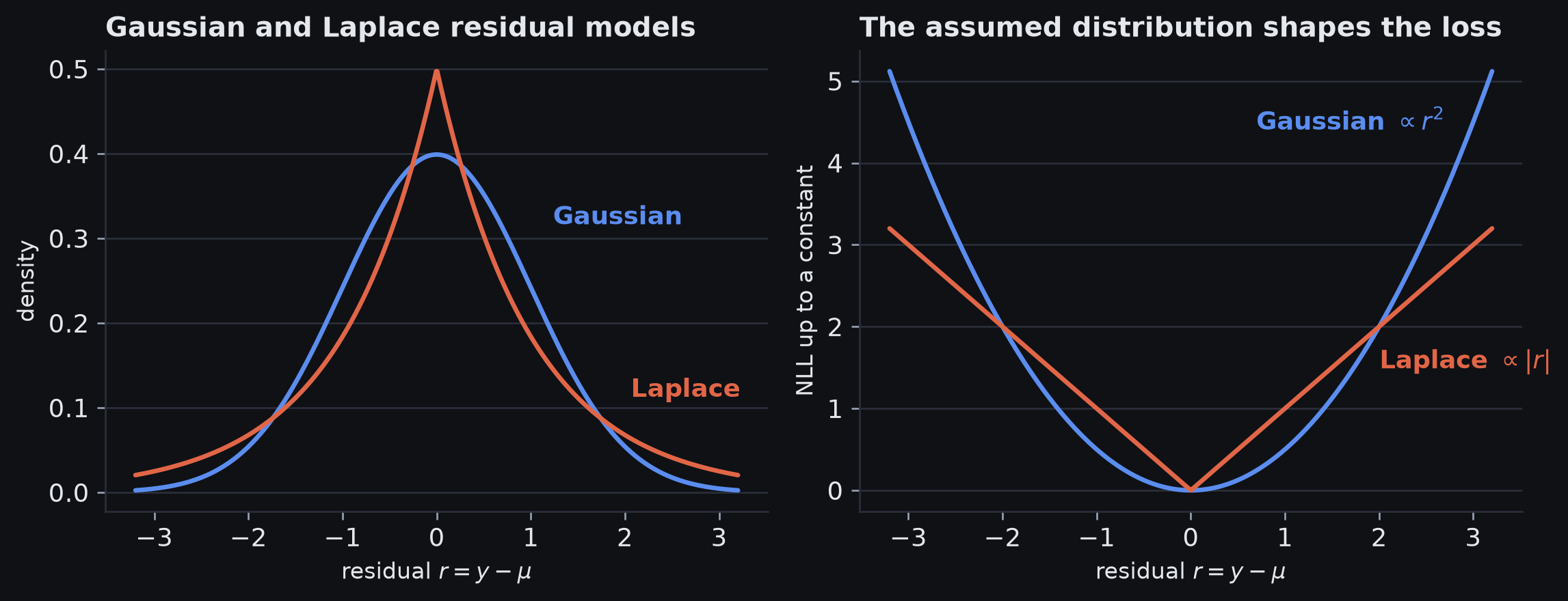
Gaussian and Laplace residual models and their corresponding NLL penalties.

Gaussian residual model \(\Rightarrow\) squared-error penalty
Laplace residual model \(\Rightarrow\) absolute-error penalty
The distributional assumption determines how residuals are weighted by the loss.

Least squares and likelihood: two fits compared

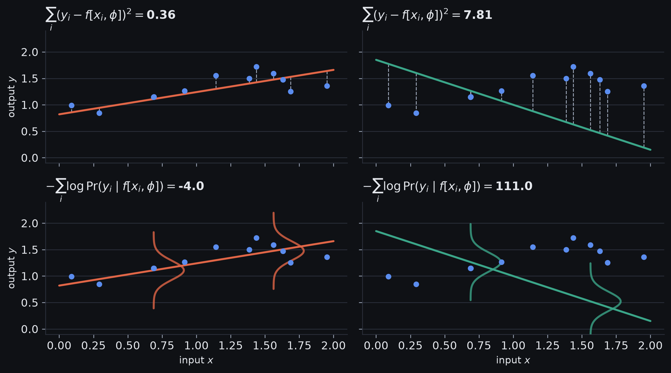
Squared-error and Gaussian-NLL scores for the same two fits. Both criteria rank the left fit better.

Least squares moves 0.36 to 7.81; the NLL moves -4.0 to 111.0
For fixed \(\sigma^2\), Gaussian NLL is an increasing affine function of squared error
The two criteria therefore rank every pair of parameter settings identically
With fixed variance, squared error and Gaussian NLL therefore choose the same \(\params\).

Inference

After training, the predictive distribution for a new input is

\[ y\mid\vect{x} \sim \normal\!\left( \model[\hat{\params}]{\vect{x}}, \sigma^2 \right). \]

If we want the maximum-density point:

\[ \hat y = \argmax_{y} p\!\left(y\mid \model[\hat{\params}]{\vect{x}},\sigma^2\right) = \model[\hat{\params}]{\vect{x}}. \tag{5.12} \]

For a normal distribution, mean = median = mode, so the familiar regression prediction is recovered.

Estimating observation uncertainty

Least squares discarded \(\sigma^2\) only because it was fixed while optimising \(\params\).

We can instead learn one shared variance jointly with the network:

\[ \boxed{ \hat{\params},\hat\sigma^2 = \argmin_{\params,\sigma^2} \left[ -\sum_{i=1}^{I} \log p\!\left( y_i\mid \model{\vect{x}_i},\sigma^2 \right) \right] } \tag{5.13} \]

Read the optimisation as learning two things from the same likelihood:

\(\params\) determines the mean function \(\mu(\vect{x})\)
\(\sigma^2\) determines one global level of observation noise around that mean

At inference:

\(\model[\hat{\params}]{\vect{x}}\) gives the predicted mean
\(\hat\sigma^2\) describes observation / aleatoric uncertainty shared across inputs

Two kinds of predictive uncertainty

“Uncertain” can mean two different things.

	Aleatoric	Epistemic
Source	randomness or noise in the observation	incomplete knowledge of the model
More data?	does not necessarily remove it	can reduce it
Example	repeated sensor readings vary	few training examples in this region
Modelled by \(\sigma^2\) here?	yes	no

The Gaussian variance in this section models aleatoric / observation uncertainty: how variable \(y\) remains even when the model parameters are fixed.

Shared variance means homoscedastic uncertainty

A single learned \(\hat\sigma^2\) assumes the same observation-noise level everywhere:

\[ y_i\mid\vect{x}_i \sim \normal\!\left( \model{\vect{x}_i}, \sigma^2 \right). \]

This is homoscedastic regression:

the mean may vary with \(\vect{x}\)
the observation variance does not vary with \(\vect{x}\)
the model captures a single global level of aleatoric uncertainty

That assumption can be unrealistic when some inputs are intrinsically noisier or less predictable than others.

sensor noise that grows with the measured quantity
a manufacturing process whose intrinsic variability changes with operating conditions
future outcomes whose inherent variability grows with forecast horizon

When one variance is not enough

A constant variance assumes the vertical spread is the same everywhere. Real data can violate that directly.

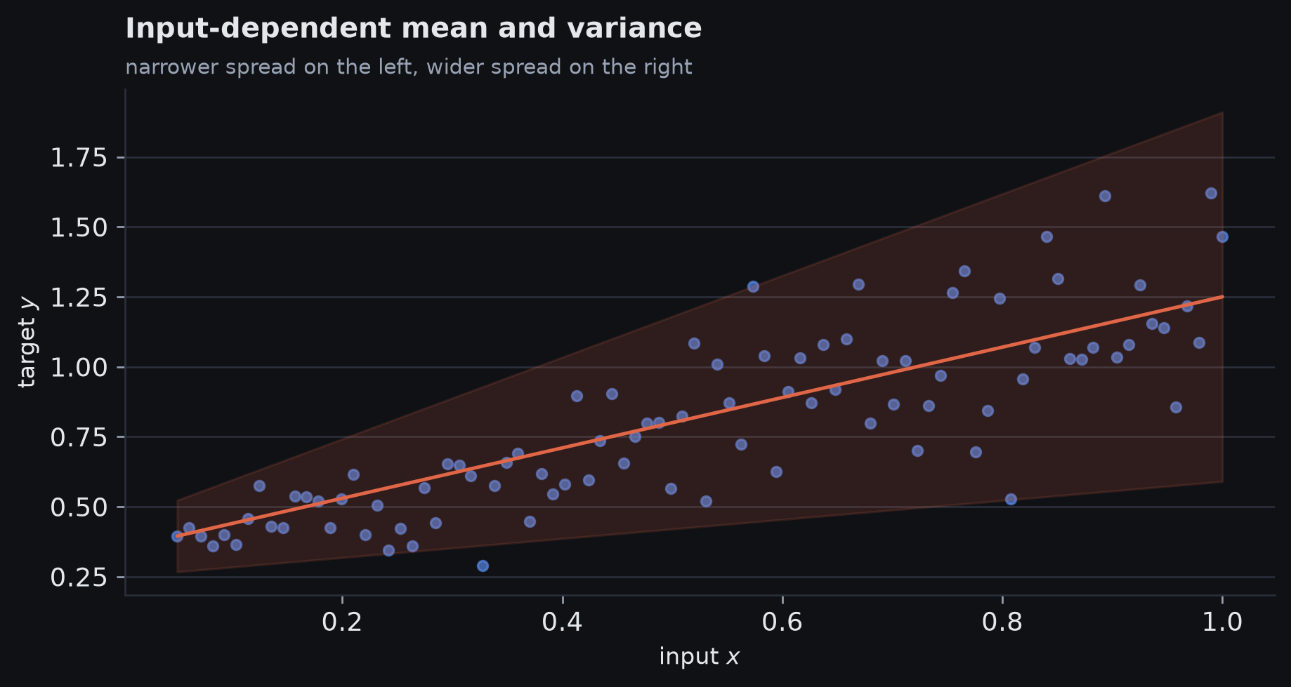
Synthetic regression data with observation variance that increases with the input.

the centre of the prediction varies with \(x\)
the irreducible spread around that centre also varies with \(x\)
heteroscedastic regression lets the model predict both

Heteroscedastic regression

If uncertainty changes with the input, model it too:

\[ \mu(\vect{x})=\mathrm{f}_1\!\left[\vect{x},\params\right], \qquad s(\vect{x})=\mathrm{f}_2\!\left[\vect{x},\params\right], \qquad \sigma^2(\vect{x})=\exp\!\left(s(\vect{x})\right). \tag{5.14} \]

Now each input gets its own predictive distribution:

\[ y\mid\vect{x} \sim \normal\!\left( \mu(\vect{x}), \sigma^2(\vect{x}) \right). \]

\(f_1\) predicts where the distribution is centred
\(f_2\) produces the unconstrained score \(s(\vect{x})\)
the exponential maps that score to a valid input-dependent variance \(\sigma^2(\vect{x})>0\)

Enforcing a valid variance

Equation 5.14 uses an unconstrained raw network output

\[ s(\vect{x})=\mathrm{f}_2\!\left[\vect{x},\params\right]\in\reals. \]

A Gaussian variance must instead be strictly positive:

\[ \sigma^2(\vect{x})>0. \]

So the raw score must be transformed before it is used as a variance:

\[ \boxed{ s(\vect{x})\in\reals \quad\longrightarrow\quad \sigma^2(\vect{x})>0 } \]

Enforcing a valid variance (cont.)

Common strictly positive parameterisations include

\[ \sigma^2(\vect{x}) = \exp\!\left(s(\vect{x})\right) \]

\[ \sigma^2(\vect{x}) = \operatorname{softplus}\!\left(s(\vect{x})\right)+\varepsilon, \]

with a small \(\varepsilon>0\) for numerical safety.

Enforcing a valid variance (cont.)

With the exponential parameterisation,

\[ s(\vect{x}) = \log \sigma^2(\vect{x}), \]

so the network directly predicts the log-variance.

With softplus, \(s(\vect{x})\) is simply an unconstrained score that is transformed into a positive variance.

The network can output any real number; the parameterisation ensures that the resulting variance is valid.

Heteroscedastic Gaussian loss

Let

\[ \mu_i=\mathrm{f}_1\!\left[\vect{x}_i,\params\right], \qquad s_i=\mathrm{f}_2\!\left[\vect{x}_i,\params\right], \qquad \sigma_i^2=\exp(s_i). \]

Then the Gaussian NLL becomes

\[ \boxed{ \loss[\params] = \sum_{i=1}^{I} \left[ \frac12\log(2\pi\sigma_i^2) + \frac{(y_i-\mu_i)^2}{2\sigma_i^2} \right] } \tag{5.15} \]

Both the mean and the variance now affect the loss for each example.

Why the variance term matters

The heteroscedastic NLL contains two competing terms:

\[ \underbrace{ \frac{(y_i-\mu_i)^2}{2\sigma_i^2} }_{\text{residual penalty}} \qquad+ \qquad \underbrace{ \frac12\log\sigma_i^2 }_{\text{uncertainty penalty}} \]

increasing \(\sigma_i^2\) makes a given residual less surprising
but predicting large variance also incurs a \(\log\sigma_i^2\) cost
the model cannot reduce the loss simply by predicting arbitrarily large variance

Together, these terms learn input-dependent variance without allowing variance to grow without penalty.

The trade-off has an interior minimum

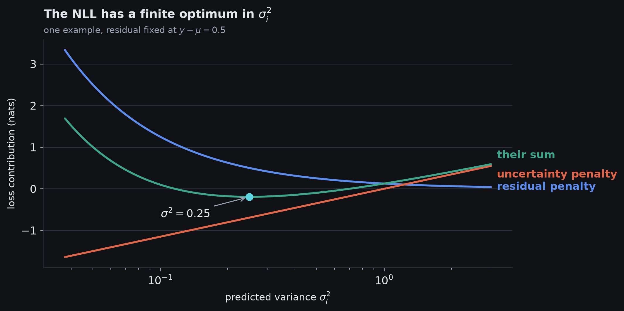
Per-example Gaussian NLL as \(\sigma_i^2\) varies for a fixed residual.

The trade-off has an interior minimum (cont.)

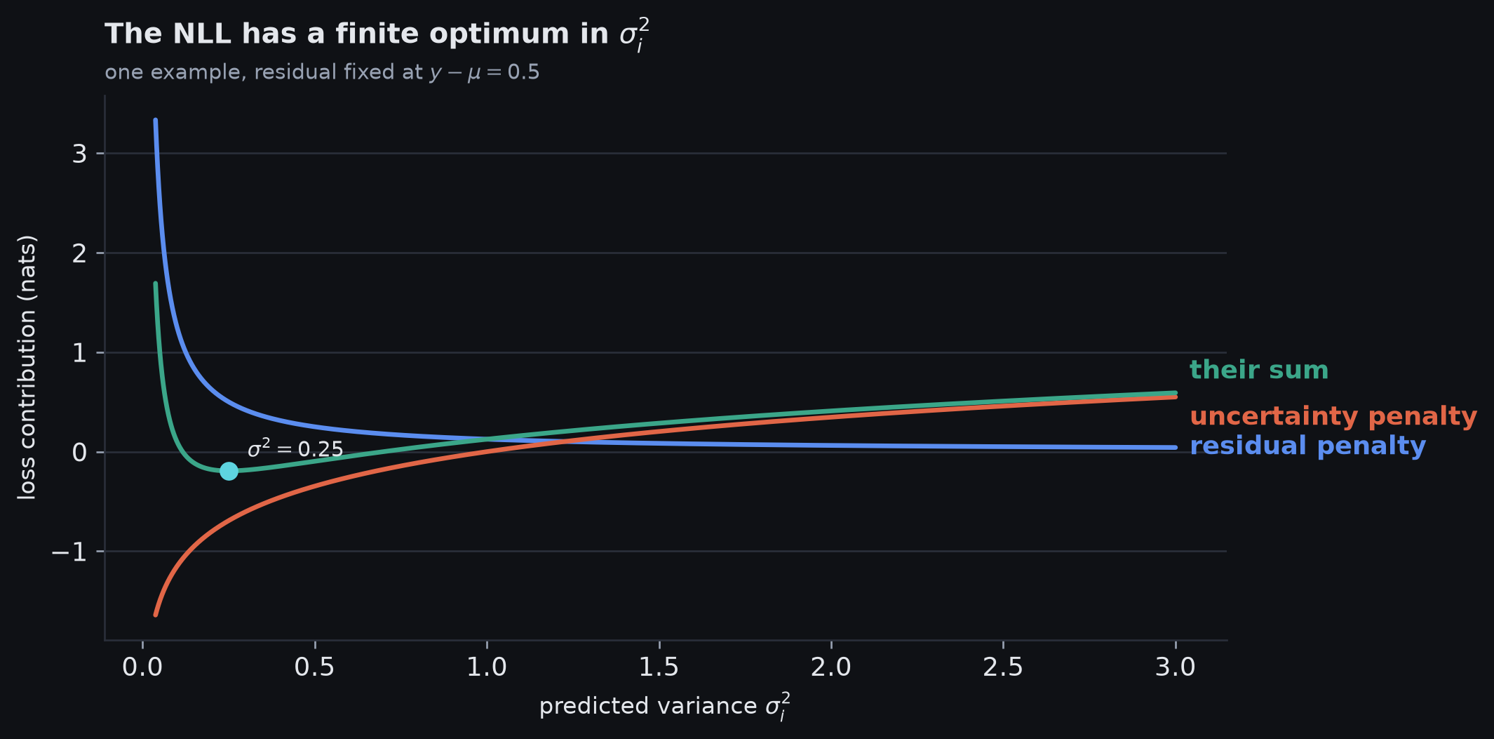
Per-example Gaussian NLL as \(\sigma_i^2\) varies for a fixed residual.

Differentiating the sum and setting it to zero gives \(\sigma_i^2=(y_i-\mu_i)^2\)
For a fixed residual, the per-example Gaussian NLL is minimised at \(\sigma_i^2=(y_i-\mu_i)^2\).

Homoscedastic vs heteroscedastic regression

	Homoscedastic	Heteroscedastic
Mean	\(\mu_i=\model{\vect{x}_i}\)	\(\mu_i=\mathrm{f}_1\!\left[\vect{x}_i,\params\right]\)
Variance	one shared \(\sigma^2\)	\(\sigma_i^2\) varies with \(\vect{x}_i\)
Network predicts	mean only	mean and an unconstrained variance score \(s\)
Uncertainty	same everywhere	input-dependent
Loss	Gaussian NLL; reduces to least squares if \(\sigma^2\) fixed	Gaussian NLL with per-example variance

Heteroscedastic regression parameterises both a conditional mean and an input-dependent variance.

Homoscedastic vs heteroscedastic networks

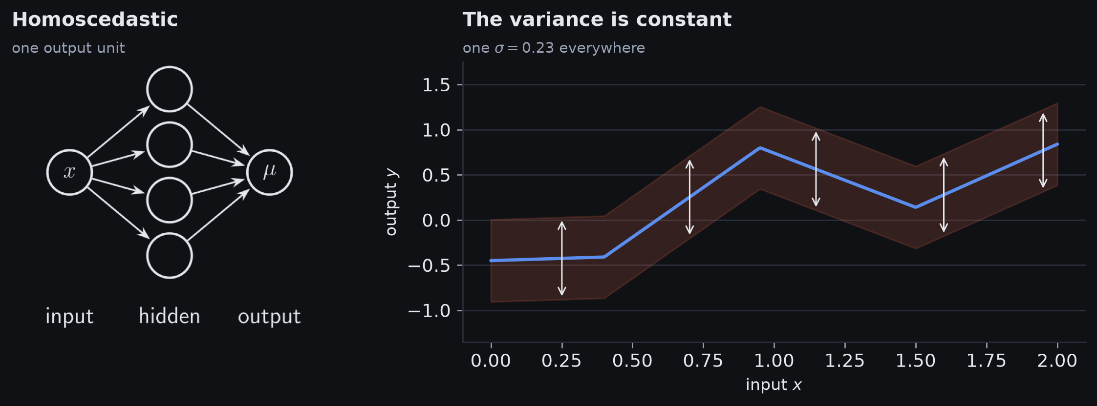
Network outputs and predictive uncertainty for homoscedastic and heteroscedastic Gaussian regression.

Homoscedastic vs heteroscedastic networks (cont.)

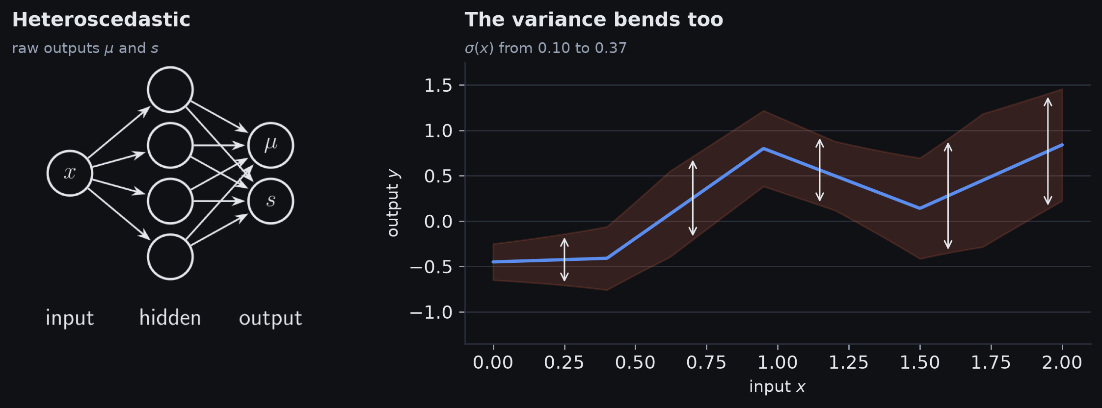
Network outputs and predictive uncertainty for homoscedastic and heteroscedastic Gaussian regression.

Regression summary

For scalar regression, a natural observation model is

\[ y\mid\vect{x}\sim\normal(\mu,\sigma^2). \]

predicting \(\mu=\model{\vect{x}}\) with fixed \(\sigma^2\) makes Gaussian NLL equivalent to least squares
learning one shared \(\sigma^2\) gives a homoscedastic uncertainty estimate
predicting \(\sigma^2(\vect{x})\) as well as \(\mu(\vect{x})\) gives heteroscedastic regression
the heteroscedastic NLL balances residual size against predicted uncertainty

\[ \boxed{ \text{choose a distribution} \rightarrow \text{predict its parameters} \rightarrow \text{NLL gives the loss} } \]

Example 2: binary classification

Apply the recipe: two classes

In binary classification, each input belongs to one of two classes:

\[ y\in\{0,1\}. \]

Here \(y\) is the class label.

Examples:

restaurant review: negative \((y=0)\) or positive \((y=1)\)
MRI scan: tumour absent \((y=0)\) or present \((y=1)\)

Following the recipe, we need a probability distribution defined on the discrete domain \(\{0,1\}\).

Step 1: choose a Bernoulli distribution

The Bernoulli distribution has one parameter

\[ \lambda\in[0,1], \]

where \(\lambda\) is the probability of class \(1\):

\[ p(y\mid\lambda) = \begin{cases} 1-\lambda, & y=0,\\[4pt] \lambda, & y=1. \end{cases} \tag{5.16} \]

Therefore

\[ p(y=1\mid\lambda)=\lambda, \qquad p(y=0\mid\lambda)=1-\lambda. \]

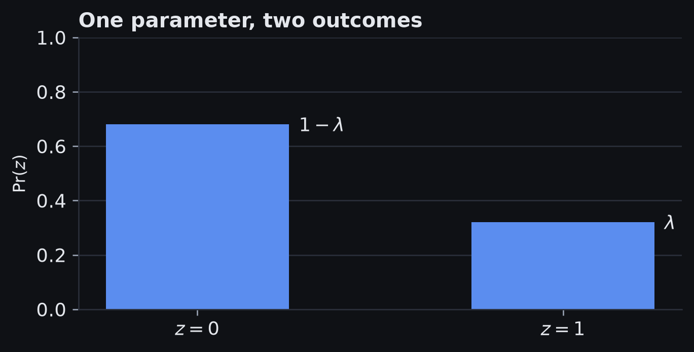
A Bernoulli distribution assigns probabilities \(1-\lambda\) and \(\lambda\) to its two outcomes.

One Bernoulli equation handles both labels

Because \(y\) is either \(0\) or \(1\), equation 5.16 can be written compactly as

\[ \boxed{ p(y\mid\lambda) = (1-\lambda)^{1-y}\lambda^y } \tag{5.17} \]

Observed label	What survives?	Likelihood
\(y=0\)	\(\lambda^0=1\)	\(1-\lambda\)
\(y=1\)	\((1-\lambda)^0=1\)	\(\lambda\)

The exponents act as switches: the observed label selects the probability assigned to the class that actually occurred.

From probability to odds to logits

A Bernoulli probability is constrained to \(0<\lambda<1\). A raw linear output unit can produce any real value.

Start with odds:

\[ \text{odds} = \frac{\lambda}{1-\lambda}. \]

Then take the logarithm:

\[ \boxed{ z = \log\frac{\lambda}{1-\lambda} } \]

This \(z\in\reals\) is the logit.

From probability to odds to logits (cont.)

Probability \(\lambda\)	Odds	Logit \(z\)
\(0.25\)	\(1:3\)	\(-\log 3\)
\(0.50\)	\(1:1\)	\(0\)
\(0.75\)	\(3:1\)	\(\log 3\)

The sigmoid is the inverse log-odds transformation: it converts an unconstrained logit back into a probability.

Step 2: sigmoid converts the logit to a probability

Let the network produce an unconstrained logit

\[ z=\model{\vect{x}}\in\reals. \]

Invert the log-odds transformation with the logistic sigmoid:

\[ \sigmoid(z) = \frac{1}{1+\exp(-z)}. \tag{5.18} \]

and define

\[ \boxed{ \lambda = \sigmoid\!\left(\model{\vect{x}}\right) } \]

Step 2: sigmoid converts the logit to a probability (cont.)

\(z=0\Rightarrow\lambda=0.5\)
\(z<0\Rightarrow\lambda<0.5\)
\(z>0\Rightarrow\lambda>0.5\)
finite \(z\) maps to \(0<\lambda<1\)

The binary predictive model

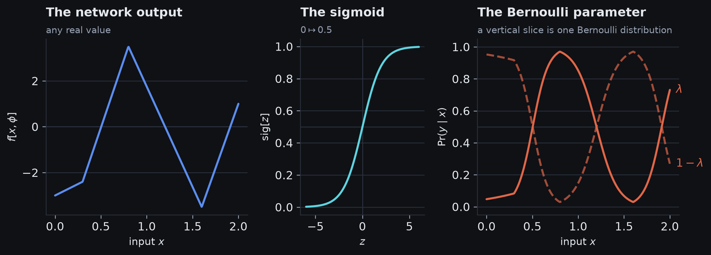
Network logit, sigmoid transformation, and resulting Bernoulli probabilities across the input.

The solid and dashed curves are one distribution, not two models
They sum to \(1\) at every input, which a hidden cell checks
The sigmoid is fixed; the learned quantity is the logit produced by the network.

Substituting \(\lambda=\sigmoid(\model{\vect{x}})\) into equation 5.17 gives

\[ \boxed{ p(y\mid\vect{x}) = \left(1-\sigmoid(\model{\vect{x}})\right)^{1-y} \sigmoid(\model{\vect{x}})^y } \tag{5.19} \]

The predictive output is a Bernoulli distribution; a class label is obtained later by thresholding.

Step 3: negative log-likelihood gives binary cross-entropy

Define

\[ \lambda_i = \sigmoid\!\left(\model{\vect{x}_i}\right). \]

For one observation,

\[ -\log p(y_i\mid\vect{x}_i) = -\log\!\left[(1-\lambda_i)^{1-y_i}\lambda_i^{y_i}\right] \]

\[ = -(1-y_i)\log(1-\lambda_i) -y_i\log\lambda_i. \]

Summing over the dataset gives

\[ \boxed{ \loss[\params] = \sum_{i=1}^{I} \left[ -(1-y_i)\log(1-\lambda_i) -y_i\log\lambda_i \right] } \tag{5.20} \]

This is the binary cross-entropy (BCE) loss. We will explain the cross-entropy terminology later.

BCE is the NLL of the observed label

For a single example:

True label	Per-example loss
\(y=1\)	\(-\log\lambda\)
\(y=0\)	\(-\log(1-\lambda)\)

\[ \exloss_i = -\log p(y_i\mid\vect{x}_i). \]

BCE is the NLL of the observed label (cont.)

For example:

Probability assigned to the true class	NLL / BCE contribution
\(0.90\)	\(0.105\)
\(0.50\)	\(0.693\)
\(0.10\)	\(2.303\)
\(0.01\)	\(4.605\)

Confidently assigning very little probability to the true class is penalised heavily.

The shape of the BCE loss

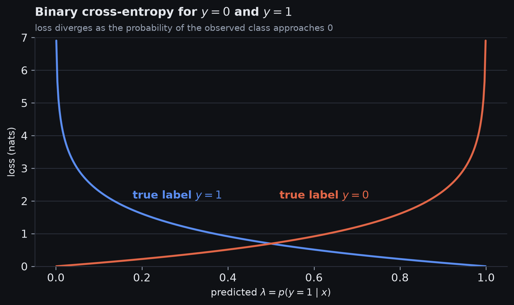
Binary cross-entropy as a function of the predicted probability for \(y=0\) and \(y=1\).

Getting from \(0.9\) to \(0.99\) saves about 0.10 nats
Going from \(0.1\) to \(0.01\) costs about 2.30 nats
Confident mistakes incur much larger BCE than uncertain predictions.

Effect of BCE on the logits

For each training example, let

\[ \lambda_i = p(y=1\mid\vect{x}_i). \]

Then maximum likelihood encourages:

\(y_i=1\Rightarrow\lambda_i\rightarrow1\)
\(y_i=0\Rightarrow\lambda_i\rightarrow0\)

Equivalently, the network learns a real-valued score \(z_i=\model{\vect{x}_i}\) such that:

positive examples tend to receive larger logits
negative examples tend to receive smaller logits
the sigmoid converts those scores into valid Bernoulli probabilities

This is the probabilistic interpretation of the binary classifier: the logit is the quantity being learned, and the sigmoid is a fixed readout of it.

Step 4: inference

After training,

\[ \lambda = \sigmoid\!\left(\model[\hat{\params}]{\vect{x}}\right) = p(y=1\mid\vect{x}). \]

If we need a class label, use the maximum-probability decision:

\[ \hat y = \begin{cases} 1, & \lambda>0.5,\\[4pt] 0, & \lambda\le0.5. \end{cases} \]

Because sigmoid is monotonic and \(\sigmoid(0)=0.5\),

\[ \lambda>0.5 \quad\Longleftrightarrow\quad \model[\hat{\params}]{\vect{x}}>0. \]

\(0.5\) is the natural maximum-probability threshold here; a deployed system may choose a different threshold when the costs of false positives and false negatives differ.

Binary cross-entropy from logits

Mathematically, we have described the pipeline as

\[ z \xrightarrow{\sigmoid} \lambda \xrightarrow{\text{BCE}} \exloss. \]

Numerically, explicitly computing \(\lambda\) extremely close to \(0\) or \(1\) and then taking \(\log\lambda\) or \(\log(1-\lambda)\) can be unstable.

training libraries therefore commonly provide a fused BCE-from-logits operation
it computes the same Bernoulli NLL
numerically it avoids unnecessary loss of precision

Logits are unconstrained real scores; sigmoid outputs are probabilities.

Binary classification summary

Binary classification has labels \(y\in\{0,1\}\)
Model uncertainty with a Bernoulli distribution
The network produces a real-valued logit and sigmoid maps it to

\[ \lambda = p(y=1\mid\vect{x}) = \sigmoid\!\left(\model{\vect{x}}\right). \]

Bernoulli negative log-likelihood is the binary cross-entropy loss

\[ \boxed{ \exloss = -(1-y)\log(1-\lambda)-y\log\lambda } \]

inference can return the probability \(\lambda\) or convert it to a class label using a decision threshold

\[ \boxed{ \text{Bernoulli model} +\text{sigmoid parameterisation} \Longrightarrow \text{binary cross-entropy} } \]

Example 3: multiclass classification

Multiclass classification: the setting

The goal is to assign an input example \(\vect{x}\) to one of \(K>2\) classes:

\[ y\in\{1,2,\ldots,K\}. \]

Examples:

handwritten-digit recognition with \(K=10\)
next-token prediction, where the next token is chosen from a vocabulary of possible outputs

As before, we apply the same loss-construction recipe.

Step 1: choose a distribution over classes

For labels taking one of \(K\) discrete values, use a categorical distribution.

Its parameters are

\[ \lambda_1,\lambda_2,\ldots,\lambda_K, \]

where

\[ \prob{y=k}=\lambda_k. \tag{5.21} \]

These parameters must satisfy:

\(\lambda_k\in[0,1]\) for every class \(k\)
\(\sum_{k=1}^{K}\lambda_k=1\)

The categorical parameter vector

Collect the class probabilities into one vector:

\[ \classprobs = \begin{bmatrix} \lambda_1\\ \lambda_2\\ \vdots\\ \lambda_K \end{bmatrix}. \]

Interpretation:

\(\lambda_k\) is the probability assigned to class \(k\)
the full vector \(\classprobs\) is the predictive distribution over classes
exactly one class is observed, but the model expresses uncertainty across all \(K\) classes

Step 2: let the network produce \(K\) scores

Use a network with \(K\) outputs:

\[ \vect{z}=\vmodel{\vect{x}}\in\reals^K. \]

Write the components as

\[ \vect{z}= \begin{bmatrix} z_1\\z_2\\\vdots\\z_K \end{bmatrix}. \]

Step 2: let the network produce \(K\) scores (cont.)

These raw outputs are often called scores or logits.

Raw logits are not probabilities:

they can be any real numbers
they need not lie in \([0,1]\)
they need not sum to one

Softmax turns logits into probabilities

To convert logits into a valid categorical distribution, apply the softmax function.

For the \(k\)th class,

\[ \softmax_k[\vect{z}] = \frac{\exp(z_k)}{\sum_{k'=1}^{K}\exp(z_{k'})}. \tag{5.22} \]

Why this works:

exponentials ensure every numerator is positive
dividing by the sum normalises the outputs
hence every output lies in \((0,1)\) and all \(K\) outputs sum to one

Softmax: one numerical example

Take three logits

\[ \vect{z}=(2,1,0). \]

Exponentiate each score:

\[ e^{\vect{z}} \approx (7.39,\;2.72,\;1.00), \qquad \sum_k e^{z_k}\approx11.11. \]

Then divide every positive score by the same total:

\[ \softmax(\vect{z}) \approx (0.665,\;0.245,\;0.090). \]

the largest logit receives the largest probability
the outputs are now positive and sum to \(1\)
softmax turns relative scores into a probability budget over classes

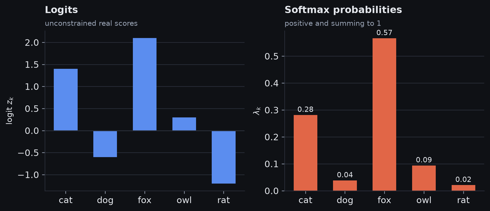
Softmax maps five logits to a categorical probability vector while preserving their ordering.

The model now predicts class probabilities

If the network produces logits

\[ \vect{z}=\vmodel{\vect{x}}, \]

then the class probabilities are

\[ \lambda_k = \softmax_k\!\left(\vmodel{\vect{x}}\right). \]

So the likelihood of label \(y=k\) is

\[ \prob{y=k\mid \vect{x}} = \softmax_k\!\left(\vmodel{\vect{x}}\right). \tag{5.23} \]

This is the multiclass analogue of the Bernoulli model used for binary classification.

Softmax probabilities across the input

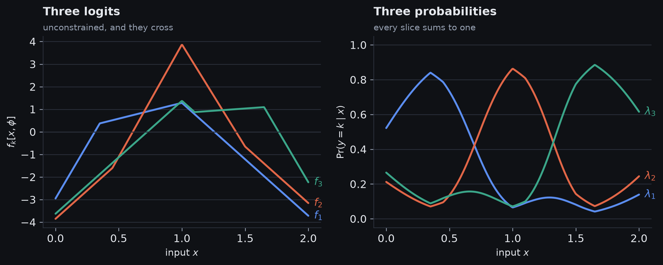
Three logits and their softmax probabilities as the input varies; each probability vector sums to one.

Softmax is applied at every input independently
The curves cross where the decision changes, not where the logits are zero
The logits reach \(\pm 4\); the probabilities top out near 0.89 — large logits are not the same as confidence
Softmax depends on differences between logits: adding the same constant to every logit leaves the probabilities unchanged.

Negative log-likelihood for multiclass labels

For a training pair \((\vect{x}_i,y_i)\), the model assigns probability to the observed class \(y_i\).

The negative log-likelihood over the dataset is

\[ \loss[\params] = -\sum_{i=1}^{I} \log\left[ \softmax_{y_i} \left(\vmodel{\vect{x}_i}\right) \right]. \]

Substituting the softmax definition gives

\[ \loss[\params] = -\sum_{i=1}^{I} \left( f_{y_i}[\vect{x}_i,\params] - \log\left[\sum_{k'=1}^{K}\exp\big(f_{k'}[\vect{x}_i,\params]\big)\right] \right). \tag{5.24} \]

Reading equation 5.24

For one training example, equation 5.24 is

\[ \exloss_i = \underbrace{-f_{y_i}[\vect{x}_i,\params]}_{\text{reward a large true-class logit}} + \underbrace{\log\!\left[\sum_{k=1}^{K}\exp(f_k[\vect{x}_i,\params])\right]}_{\text{normalise against all competing logits}}. \]

Read it in three steps:

identify the logit belonging to the true class \(y_i\)
compare it against all class logits through the log-sum-exp term
reduce the loss by making the true-class logit large relative to its competitors

Multiclass cross-entropy is therefore a competition among logits, not an independent penalty on each score.

Multiclass NLL is cross-entropy

\[ \text{categorical model} + \text{softmax parameterisation} \Longrightarrow \text{multiclass NLL / cross-entropy loss}. \]

high probability on the true class gives low loss
probability assigned to competing classes enters through the softmax normalisation
the later cross-entropy section derives this interpretation

Step 4: inference

After training, the predictive distribution is

\[ \prob{y=k\mid \vect{x}} = \softmax_k\!\left(\vmodel[\hat{\params}]{\vect{x}}\right). \]

If we want a single class label, choose the most probable class:

\[ \hat y = \argmax_{k} \prob{y=k\mid \vect{x},\hat{\params}}. \]

This is the class with the largest softmax probability at that input.

Argmax does not require softmax

Every class shares the same positive denominator. For any two classes \(j\) and \(k\),

\[ \softmax_j(\vect{z})>\softmax_k(\vect{z}) \iff \frac{e^{z_j}}{\sum_r e^{z_r}} > \frac{e^{z_k}}{\sum_r e^{z_r}} \iff z_j>z_k. \]

Therefore

\[ \boxed{ \argmax_{k}\softmax_k(\vect{z}) = \argmax_{k} z_k } \]

So for point classification:

the predicted class can be found directly from the logits
applying softmax is still useful when we want the full predictive probabilities

This is analogous to the binary fact that thresholding the sigmoid probability at \(0.5\) is equivalent to thresholding the logit at \(0\).

Predicting other data types

Regression and classification are especially common, but the recipe is more general.

To predict any other kind of output:

identify the domain of the target
choose a probability distribution defined on that domain
let the model predict the parameter(s) of that distribution
train with the corresponding negative log-likelihood

General pattern:

\[ \text{target domain} \Longrightarrow \text{distribution choice} \Longrightarrow \text{negative log-likelihood loss}. \]

Multiclass classification summary

Multiclass classification predicts one of \(K>2\) labels
Use a categorical distribution with parameters \(\lambda_1,\ldots,\lambda_K\)
A network with \(K\) outputs produces logits, and softmax maps them to valid probabilities

\[ \prob{y=k\mid\vect{x}} = \softmax_k\!\left(\vmodel{\vect{x}}\right). \]

The negative log-likelihood is the multiclass cross-entropy loss
For point prediction, choose the most probable class

\[ \boxed{ \text{categorical distribution} +\softmax \Longrightarrow \text{multiclass cross-entropy} } \]

Multiple outputs

From one target to a target vector

Often, one model must make several predictions from the same input.

Instead of a scalar target \(y\), write

\[ \vect{y} = (y_1,y_2,\ldots,y_D). \]

Examples:

predict a molecule’s melting point and boiling point
predict an object class at every image location

A full joint distribution can model dependencies between components of \(\vect{y}\).

A common simplification is to treat the output components as conditionally independent given the input.

Factorising the output distribution

Under the output-independence assumption,

\[ \prob{\vect{y}\mid \vmodel{\vect{x}}} = \prod_{d=1}^{D} \prob{y_d\mid \vect{f}_d\!\left[\vect{x},\params\right]}. \tag{5.25} \]

where:

\(d\) indexes an output component
\(y_d\) is the target for that component
\(\vect{f}_d\!\left[\vect{x},\params\right]\) denotes the network output(s) that parameterise the distribution for \(y_d\)

This is a modelling assumption, not something guaranteed by using a neural network.

Example: multiple continuous outputs

Suppose every target component is real-valued:

\[ y_d\in\reals. \]

A simple model uses one Gaussian for each output:

\[ y_d\mid\vect{x} \sim \normal(\mu_d,\sigma_d^2), \qquad \mu_d=\vect{f}_d\!\left[\vect{x},\params\right]. \]

the network predicts one mean for each quantity
the variances may be fixed, learned globally, or predicted from the input
with fixed equal variances, the resulting NLL reduces to a sum of squared errors across outputs

Example: multiple discrete outputs

Suppose each output component is a \(K\)-class label:

\[ y_d\in\{1,2,\ldots,K\}. \]

Use one categorical distribution for each \(y_d\).

For output component \(d\), the network must produce \(K\) logits:

\[ \vect{f}_d\!\left[\vect{x},\params\right] = \big(z_{d1},z_{d2},\ldots,z_{dK}\big). \]

Softmax converts those logits into the categorical probabilities for that component.

So a multi-output classifier may contain one group of logits per predicted label.

Negative log-likelihood becomes a double sum

For training example \(i\), write \(y_{id}\) for output component \(d\).

\[ \loss[\params] = -\sum_{i=1}^{I} \sum_{d=1}^{D} \log \prob{y_{id}\mid \vect{f}_d\!\left[\vect{x}_i,\params\right]}. \tag{5.26} \]

Read the two sums from the inside out:

\(-\log p(\cdot)\) is the surprise for one output of one example
\(\sum_d\) adds the surprises across that example’s output components
\(\sum_i\) then adds them across training examples

\[ \boxed{\text{total loss} = \text{sum over examples of the sum over outputs}} \]

The additive form comes directly from the conditional-independence factorisation.

Why the output losses add

The same product-to-sum rule appears again.

For one training example:

\[ \prob{\vect{y}\mid\vect{x}} = \prod_{d=1}^{D}\prob{y_d\mid\vect{x}}. \]

Taking negative logs gives

\[ -\log\prob{\vect{y}\mid\vect{x}} = -\sum_{d=1}^{D}\log\prob{y_d\mid\vect{x}}. \]

So independent output distributions imply additive per-output NLL terms.

The outputs can have different types

The components of \(\vect{y}\) do not need to share the same domain or distribution.

Example: predict both wind direction and wind strength.

Output	Domain	Possible distribution
direction	\((-\pi,\pi]\)	von Mises
strength	\(\reals_{+}\)	exponential

Under conditional independence,

\[ \prob{\text{direction},\text{strength}\mid\vect{x}} = \prob{\text{direction}\mid\vect{x}} \prob{\text{strength}\mid\vect{x}}. \]

Their negative log-likelihood terms then add in the training loss.

Choosing distributions: continuous targets

The maximum-likelihood recipe extends well beyond Gaussian regression.

Target/domain	Distribution	Typical use
\(y\in\reals\)	normal	ordinary univariate regression
\(y\in\reals\)	Laplace or \(t\)	robust regression
\(y\in\reals\)	mixture of Gaussians	multimodal regression
\(y\in\reals_{+}\)	exponential or gamma	positive magnitudes

Choosing distributions: continuous targets (cont.)

Target/domain	Distribution	Typical use
\(y\in[0,1]\)	beta	proportions
\(\vect{y}\in\reals^K\)	multivariate normal	correlated multivariate regression
\(y\in(-\pi,\pi]\)	von Mises	circular direction

The target domain constrains the candidate distributions; modelling assumptions decide which one to use.

Choosing distributions: discrete and structured targets

Target/domain	Distribution	Typical use
\(y\in\{0,1\}\)	Bernoulli	binary classification
\(y\in\{1,\ldots,K\}\)	categorical	multiclass classification
\(y\in\{0,1,2,\ldots\}\)	Poisson	event counts
\(\vect{y}\in\operatorname{Perm}(1,\ldots,K)\)	Plackett–Luce	rankings / permutations

The general recipe remains unchanged:

\[ \text{domain} \Longrightarrow \text{distribution} \Longrightarrow \text{parameterisation} \Longrightarrow \text{NLL}. \]

Limits of independence

The factorisation in equation 5.25 is convenient, but it discards dependencies between outputs.

For example:

melting point and boiling point may be correlated
neighbouring image labels are often correlated
several measurements may rise or fall together

If these dependencies matter, a product of independent univariate distributions may be inadequate.

Then we may need a joint multivariate or structured distribution that models relationships between outputs explicitly.

Independence is therefore a simplification of the statistical model, not a statement that the real outputs are unrelated.

If outputs are correlated: model them jointly

For several continuous outputs, one alternative is a multivariate normal:

\[ \vect{y}\mid\vect{x} \sim \normal\!\left(\mean(\vect{x}),\mat{\Sigma}(\vect{x})\right). \]

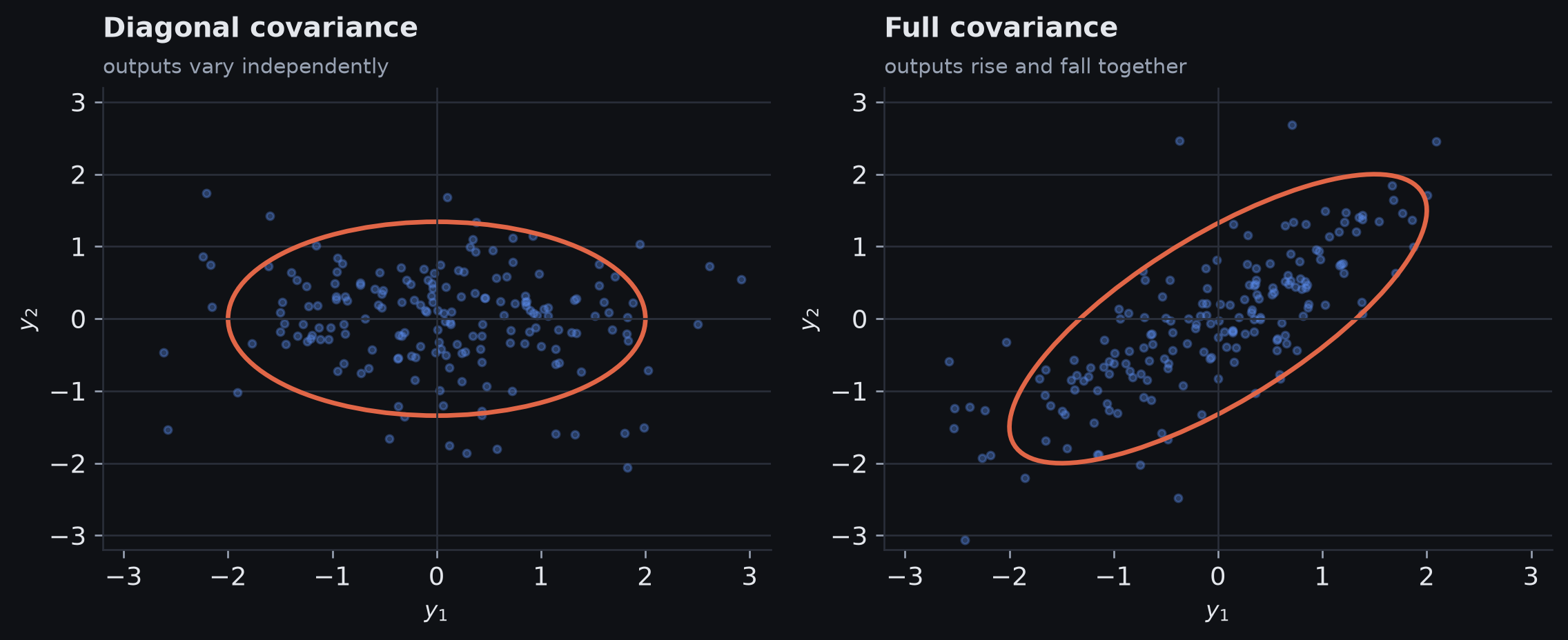
Two bivariate Gaussian models: diagonal covariance gives an axis-aligned ellipse; non-zero covariance tilts it.

diagonal \(\mat{\Sigma}\): no covariance terms; Gaussian components factorise
full \(\mat{\Sigma}\): off-diagonal terms represent outputs varying together
the ellipse’s tilt is the visual signature of covariance

\[ \text{independent per-output distributions} \quad\text{vs}\quad \text{one joint distribution} \]

Use the simpler factorisation when adequate; use a joint model when dependencies are part of what must be predicted.

Multiple outputs summary

A model can predict a vector of outputs

\[ \vect{y}=(y_1,\ldots,y_D). \]

A common simplification is to treat output components as conditionally independent

\[ \prob{\vect{y}\mid\vect{x}} = \prod_{d=1}^{D}\prob{y_d\mid\vect{x}}. \]

Negative log-likelihood converts the product into an additive loss

\[ \boxed{ \loss[\params] = -\sum_i\sum_d \log\prob{y_{id}\mid \vect{f}_d\!\left[\vect{x}_i,\params\right]} } \]

Different outputs may use different distributions
When output dependencies matter, model a joint distribution rather than assuming independence

Cross-entropy loss

Why another view of the loss?

We already have a training objective:

\[ \loss[\params] = -\sum_i \log p\!\left(y_i\mid \model{\vect{x}_i}\right). \]

Why another view of the loss? (cont.)

The same fitting problem can be viewed in several ways:

View	Question
Negative log-likelihood	How well did the model score the observations we actually saw?
Cross-entropy	How well would the model score outcomes generated by the data distribution?
KL divergence	How much extra log-loss comes from the model distribution not matching the data distribution?

These are not three competing losses in this setting. They are closely related views of the same fitting problem.

Start with something familiar: surprise

For a discrete observed outcome \(y\), we already used

\[ \boxed{\text{surprise}(y)=-\log p(y)}. \]

Probability assigned to the outcome	Surprise \(-\log p\)
\(0.9\)	\(0.105\)
\(0.5\)	\(0.693\)
\(0.1\)	\(2.303\)
\(0.01\)	\(4.605\)

likely outcomes are unsurprising
unlikely outcomes are surprising
this is the same quantity that appears in each NLL term

Entropy: average surprise under one distribution

Suppose outcomes are generated by a distribution \(q\).

Before observing the next outcome, some distributions are much more predictable than others.

if one outcome has almost all the probability, there is little uncertainty
if probability is spread across many outcomes, there is more uncertainty

Entropy is the average surprise when outcomes are drawn from \(q\) and scored using \(q\) itself:

\[ \boxed{ H(q) = \expectsub{Y\sim q}{-\log q(Y)} } \]

Entropy is a property of the distribution, not of one particular observed value.

Low entropy and high entropy

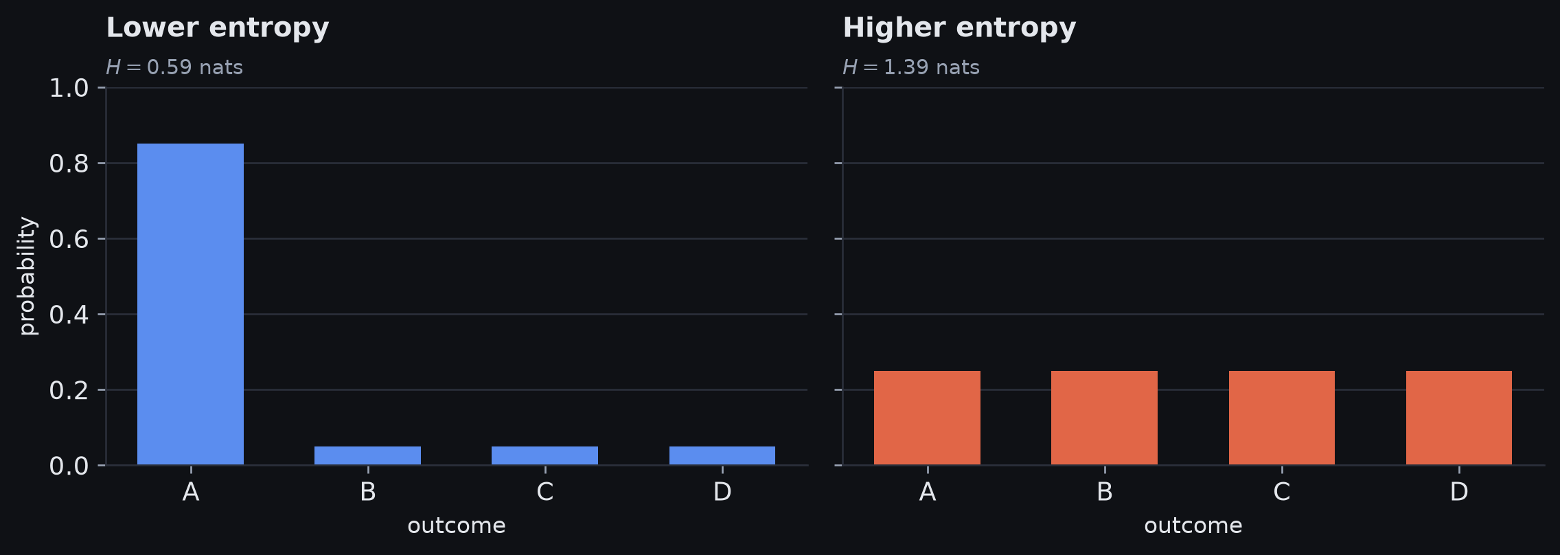
Two distributions over four outcomes. Concentrated probability gives lower entropy; more evenly spread probability gives higher entropy.

low entropy: most probability is concentrated on a small number of outcomes
high entropy: more outcomes remain plausible before we observe the result
with natural logarithms, entropy is measured in nats; base-\(2\) logarithms give bits

In security, people often speak loosely of a high-entropy key or password. More precisely, the entropy belongs to the source or distribution it was drawn from: many plausible outputs mean greater uncertainty before the value is known.

From entropy to cross-entropy

Now distinguish two distributions:

\(q(y)\) — the distribution that generates the data
\(p(y)\) — the distribution predicted by our model

For the moment we suppress the input \(x\) to keep the notation simple. In supervised learning, these become conditional distributions such as \(q(y\mid x)\) and \(p(y\mid x)\).

There are now two ways to score outcomes drawn from \(q\):

\[ \begin{aligned} H(q) &= \expectsub{Y\sim q}{-\log q(Y)} &&\text{score }q\text{ using }q,\\[6pt] \xent{q}{p} &= \expectsub{Y\sim q}{-\log p(Y)} &&\text{score }q\text{ using }p. \end{aligned} \]

Entropy: how uncertain the data are intrinsically.
Cross-entropy: how surprised model \(p\) is, on average, by data drawn from \(q\).

Worked example: cross-entropy

Suppose the data distribution is \(q\), while the model predicts \(p\):

Outcome \(y\)	\(q(y)\)	\(p(y)\)	Model surprise \(-\log p(y)\)	Weighted surprise \(q(y)[-\log p(y)]\)
1	\(0.50\)	\(0.60\)	\(0.511\)	\(0.255\)
2	\(0.30\)	\(0.30\)	\(1.204\)	\(0.361\)
3	\(0.20\)	\(0.10\)	\(2.303\)	\(0.461\)

Add the weighted surprises:

\[ \xent{q}{p} \approx 0.255+0.361+0.461 = 1.077\ \text{nats}. \]

Worked example: what cross-entropy is averaging

\(q(y)\) says how often each outcome contributes to the average
\(-\log p(y)\) says how surprising the model finds that outcome
a common outcome given very little model probability contributes strongly to the cross-entropy

\[ \boxed{ \text{cross-entropy} = \text{average model surprise on data from }q } \]

Entropy, cross-entropy, and KL divergence

Cross-entropy contains two conceptually different sources of log-loss:

\[ \boxed{ \xent{q}{p} = H(q) + \kl{q}{p} } \]

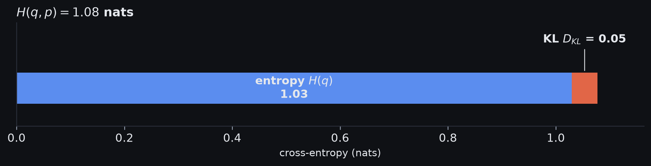
Cross-entropy decomposed into entropy plus KL divergence for the worked example.

What the decomposition means

\(H(q)\) — intrinsic uncertainty

Even a perfect model cannot make the underlying data-generating process more predictable than it is.

\(D_{\mathrm{KL}}(q\|p)\) — model mismatch

This is the extra expected log-loss caused by using \(p\) instead of \(q\).

\[ \boxed{ \kl{q}{p} = \text{cross-entropy} - \text{entropy} } \]

KL divergence is the part of the cross-entropy attributable to model mismatch.

Why minimising cross-entropy minimises KL divergence

When fitting the model, \(q\) is fixed. Changing the model changes \(p\), not the data-generating distribution.

Therefore \(H(q)\) is constant with respect to the model parameters:

\[ \xent{q}{p} = \underbrace{H(q)}_{\text{fixed}} + \underbrace{\kl{q}{p}}_{\text{changes with }p}. \]

Hence

\[ \boxed{ \argmin_p \xent{q}{p} = \argmin_p \kl{q}{p} } \]

We cannot reduce the intrinsic uncertainty in \(q\); fitting can only reduce the mismatch between \(p\) and \(q\).

KL divergence: formal definition

For discrete outcomes,

\[ \boxed{ \kl{q}{p} = \sum_y q(y) \log\frac{q(y)}{p(y)} } \]

Read one term from right to left:

\(q(y)/p(y)\) compares the probability assigned by the two distributions
the logarithm turns that ratio into a log-score difference
multiplying by \(q(y)\) gives more weight to outcomes that occur more often under \(q\)
summing averages that mismatch across possible outcomes

The formula formalises the idea we already have: average extra log-loss caused by using \(p\) instead of \(q\).

KL divergence for continuous outcomes

For continuous outcomes, probability masses become densities and the sum becomes an integral:

\[ \kl{q}{p} = \int q(y) \log\frac{q(y)}{p(y\mid\distparams)}\,dy. \tag{5.27} \]

the same weighting idea applies: mismatches matter most where \(q\) places density
\(\kl{q}{p}\ge0\)
KL divergence is generally not symmetric

For continuous variables, the corresponding entropy is differential entropy. We use the same cross-entropy/NLL connection here, but differential entropy does not share every property of discrete Shannon entropy.

KL divergence is directional

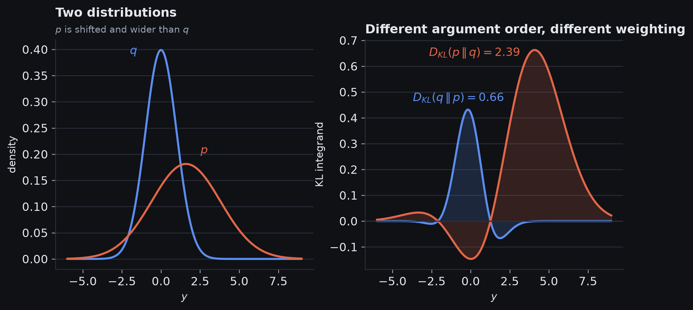
KL divergence for the same two distributions in both argument orders.

\(D_{\mathrm{KL}}(q\|p)\) weights mismatches according to where \(q\) places density
reversing the arguments changes which distribution supplies those weights
therefore \(D_{\mathrm{KL}}(q\|p)\) and \(D_{\mathrm{KL}}(p\|q)\) generally differ

From the population to the training set

The true data distribution \(q\) is unknown. We only observe training examples drawn from it.

Population cross-entropy is an expectation:

\[ \xent{q}{p} = \expectsub{Y\sim q}{-\log p(Y)}. \]

Estimate that expectation with the sample average:

\[ \xent{q}{p} \approx -\frac{1}{I} \sum_{i=1}^{I} \log p(y_i). \]

\[ \boxed{ \text{expected model surprise} \longrightarrow \text{average surprise on observed data} } \]

Empirical samples and model scores

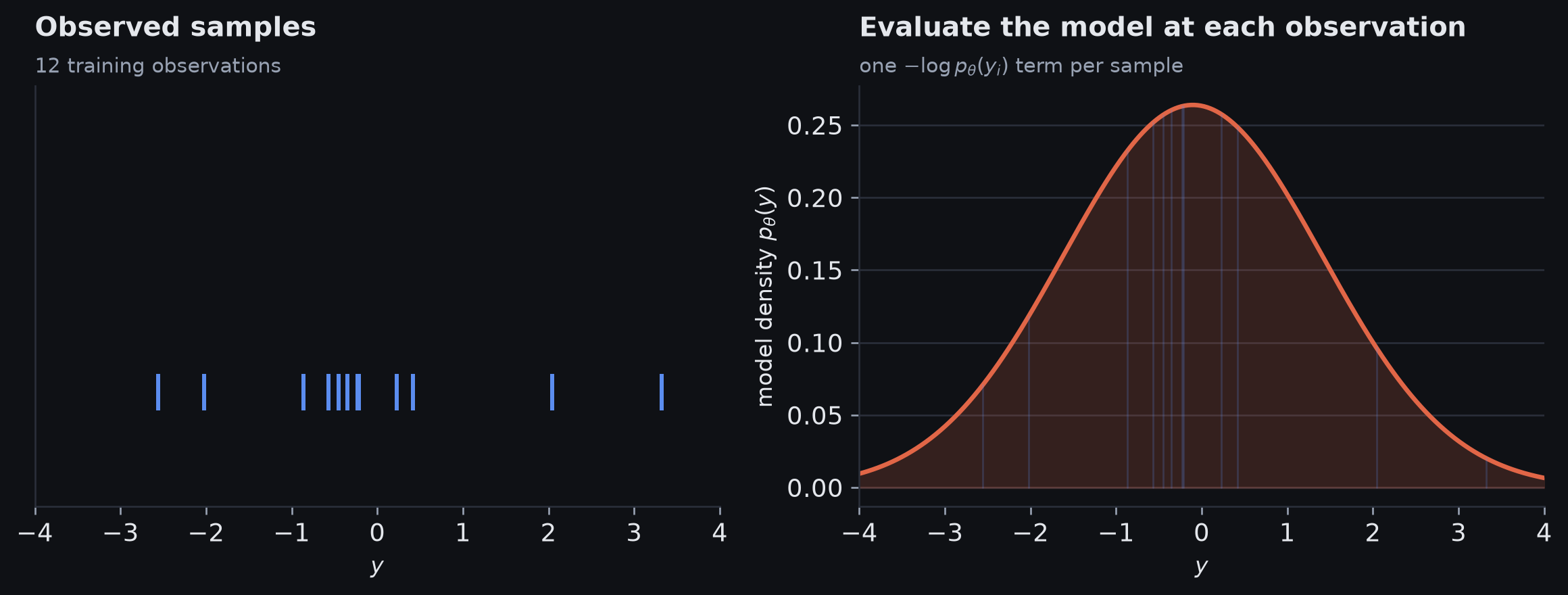
Observed samples and the model density evaluated at those samples.

evaluate the model mass or density at every observed \(y_i\)
convert each score to \(-\log p(y_i)\)
average those terms over the sample

That sample average is empirical cross-entropy; it is also the mean negative log-likelihood.

Cross-entropy and NLL are the same objective here

Return now to supervised learning, where the predictive distribution depends on the input. In population form, the corresponding cross-entropy averages \(-\log p(Y\mid X)\) over input-target pairs \((X,Y)\) drawn from the data distribution.

For the training set, the network supplies the distribution parameters for each observed input:

\[ \distparams_i = \model{\vect{x}_i}. \]

The empirical cross-entropy is therefore

\[ -\frac1I \sum_{i=1}^{I} \log p\!\left(y_i\mid\model{\vect{x}_i}\right). \]

Apart from the positive scale factor \(1/I\), this is exactly the NLL used throughout the lecture:

\[ \boxed{ \text{minimum empirical cross-entropy} \Longleftrightarrow \text{minimum NLL} \Longleftrightarrow \text{maximum likelihood} } \]

Same arithmetic, different viewpoint

Viewpoint	What is held conceptually in focus?	Quantity
Maximum likelihood / NLL	the observed training examples	log-loss on the observed targets
Cross-entropy	the data distribution and model distribution	expected model log-loss under the data distribution
KL divergence	mismatch between the two distributions	cross-entropy minus the entropy of the data distribution

In this supervised maximum-likelihood setting, cross-entropy does not introduce a second loss to optimise. It explains the same objective as distribution matching.

Why the classification losses are called cross-entropy

Binary classification

\[ \exloss = -y\log\lambda-(1-y)\log(1-\lambda) \]

is both Bernoulli negative log-likelihood and binary cross-entropy.

Multiclass classification

\[ \exloss=-\log\lambda_y \]

is both categorical negative log-likelihood and multiclass cross-entropy.

The formula is the same; NLL and cross-entropy describe two ways of interpreting it.

Retrieval practice

What changes when we reinterpret \(\model{\vect{x}}\) as distribution parameters rather than a direct prediction?
Which assumption lets a dataset likelihood become a product of per-example likelihoods?
Why does a Gaussian model with fixed variance produce least-squares loss?
What is the difference between homoscedastic and heteroscedastic observation uncertainty?
Why do binary and multiclass classifiers need sigmoid and softmax parameterisations?
Why does independent multi-output modelling produce a sum of per-output losses?
In words, what is the difference between entropy, cross-entropy, and KL divergence?
Why are maximum likelihood, minimum NLL, and minimum empirical cross-entropy the same training objective here, and why does minimising population cross-entropy also minimise \(D_{\mathrm{KL}}(q\|p)\)?

Summary

From model architecture to loss function

We started with families of functions

\[ \model{\vect{x}}. \]

The loss function answers:

How do we decide which parameter setting is best?

Interpret the network as predicting parameters of a probability distribution:

\[ \distparams = \model{\vect{x}}, \qquad y\sim p(y\mid\distparams). \]

Loss-function recipe

For a new prediction problem:

identify the target domain
choose a suitable probability distribution on that domain
let the network predict its parameter(s)
evaluate the observed targets under that distribution
minimise negative log-likelihood

\[ \boxed{ \loss[\params] = -\sum_i \log p\!\left(y_i\mid \model{\vect{x}_i}\right) } \]

The distributional assumptions determine the concrete form of the loss.

What the common losses mean

Prediction problem	Distribution	Parameterisation	Resulting loss
real-valued regression	normal	predicted mean	least squares
binary classification	Bernoulli	sigmoid probability	binary cross-entropy
multiclass classification	categorical	softmax probabilities	multiclass cross-entropy
multiple outputs	product of chosen distributions	one parameter set per output	sum of per-output NLLs

What the common losses mean (cont.)

Extensions include:

learning predictive variance
heteroscedastic uncertainty
mixed output types
joint distributions when independence is inappropriate

Fitting: likelihood and cross-entropy

Likelihood view

\[ \text{choose parameters that make the observed data likely} \]

Cross-entropy view

\[ \text{minimise average model log-loss on the empirical data distribution} \]

Both give the same optimisation criterion:

\[ \boxed{ \text{maximum likelihood} \Longleftrightarrow \text{minimum NLL} \Longleftrightarrow \text{minimum empirical cross-entropy} } \]

Next: optimisation

A learning problem now has two pieces:

a model \(\model{\vect{x}}\)
a loss \(\loss[\params]\) that scores its parameters

The remaining question is computational:

\[ \boxed{ \text{How do we find } \hat{\params} = \argmin_{\params} \loss[\params]? } \]

That is the subject of the next chapter: model training and optimisation.

Questions?

Eoin O’Brien · eoin@eoin.ai